Causal inference is the set of methods for estimating how an outcome would change if we changed one thing while holding everything else constant.
The best way to understand causal inference and apply it in practice is through a practical example, not to get overwhelmed by theory. For this purpose, let’s use an example of a retailer that launched a loyalty program. Six months later, we want to assess the program’s effectiveness. An initial report shows that loyalty program users spend 23.5 EUR more than other customers.
But in reality, the program increases each member’s average spend by around 6 EUR. The remaining initial gap comes from self-selection bias. Customers who already spent the most often signed up for the program. Both numbers come from the same data, but only one of them tells you what the programme did.
Causal inference closes that gap. This guide gives readers a basic understanding of causal inference and how to use it. We will see why simple comparison fails, what a counterfactual is, the main methods, and which assumptions we cannot skip.
Causal inference in one sentence
Causal inference estimates what would happen to an outcome if we intervened in one of its causes. In causal inference, we call that intervention a treatment, and our main task is to estimate its effect.
The crucial word here is ‘intervened’, because it takes us out of the descriptive world. Most analyses focus on describing the data we already have and plotting trends, revenue per customer, sales history and so on. All of it is valuable, but it keeps us at the simplest approach. In short, those patterns are correlations. They hold only as long as the world keeps running the way it did when we collected the data.
Two questions related to the loyalty program example show the difference between descriptive and causal worlds:
- Descriptive question: How much more do loyalty members spend than non-members?
- Causal question: How much more would a customer spend if we enrolled them?
We can answer both using the data we already have. To answer the first question, we only need to check simple averages per group. The second question requires something we didn’t observe: what each member would have spent without the programme. That missing outcome is the counterfactual, and estimating it is the core task of causal inference.
A causal inference example: does a loyalty programme raise spend?
Let’s follow up on our example to better understand the problem in practice. We simulated the data for the retailer with 10,000 customers. As mentioned in the introduction, the company launched a free loyalty program. Members earn points on every order and get early access to promotions. Joining is optional, and each customer sees an invitation in the app and decides for themselves. We also assume that the company is fully digital so that we can track each transaction at the customer level. For educational purposes, this example is of course simplified, as our main goal is to highlight the need for causality, not to get trapped in technical details.
Six months later, the board asks whether the program is worth the cost. We have the following fields available for every customer:
- Prior spend – Average monthly spend in the six months before launch.
- Member – Whether the customer joined the loyalty program
- Spend after the start – Average monthly spend after the program launched.
We built this dataset with a simulation, on purpose. In real data, the true effect is unknown, so nobody can say which estimate is right. We set the rule ourselves: membership adds exactly €6 a month to each member’s spend.
Out of 10,000 customers, 3,434 joined. The analytics team compared the two groups and found that members spend far more than non-members.
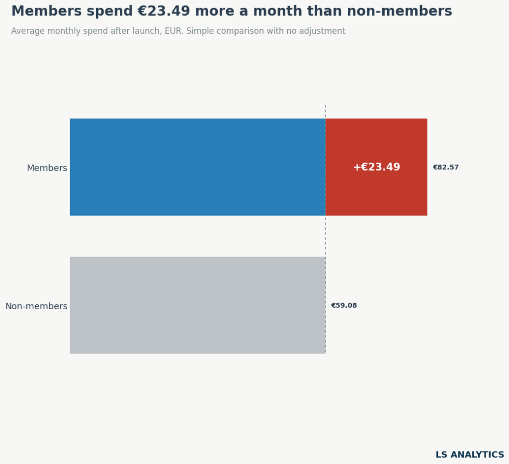
The results seemingly speak for themselves. Members spend about €23.50 more per month. Multiply that by 3,434 members, and the programme appears to bring in over €80,000 a month.
Why the simple comparison is wrong
Members and non-members were different customers even before the program started. In the six months before launch, members already spent an average of €72 a month, while non-members spent €54. The difference has nothing to do with joining a loyalty program; it reflects the two groups’ different characteristics.
Customers who joined a loyalty scheme spend more and shop more often. This also means they stand to gain the most from a reward-based loyalty scheme. As they spend more, they will also gain the most from the points customers receive after shopping. It makes the composition of customers joining the program skewed in favour of the higger value group. Among the lowest value customers, 9% joined, while almost 80% of higher spenders joined the program. As the chart below shows, the higher the spend before the program launched, the more likely a customer is to join.
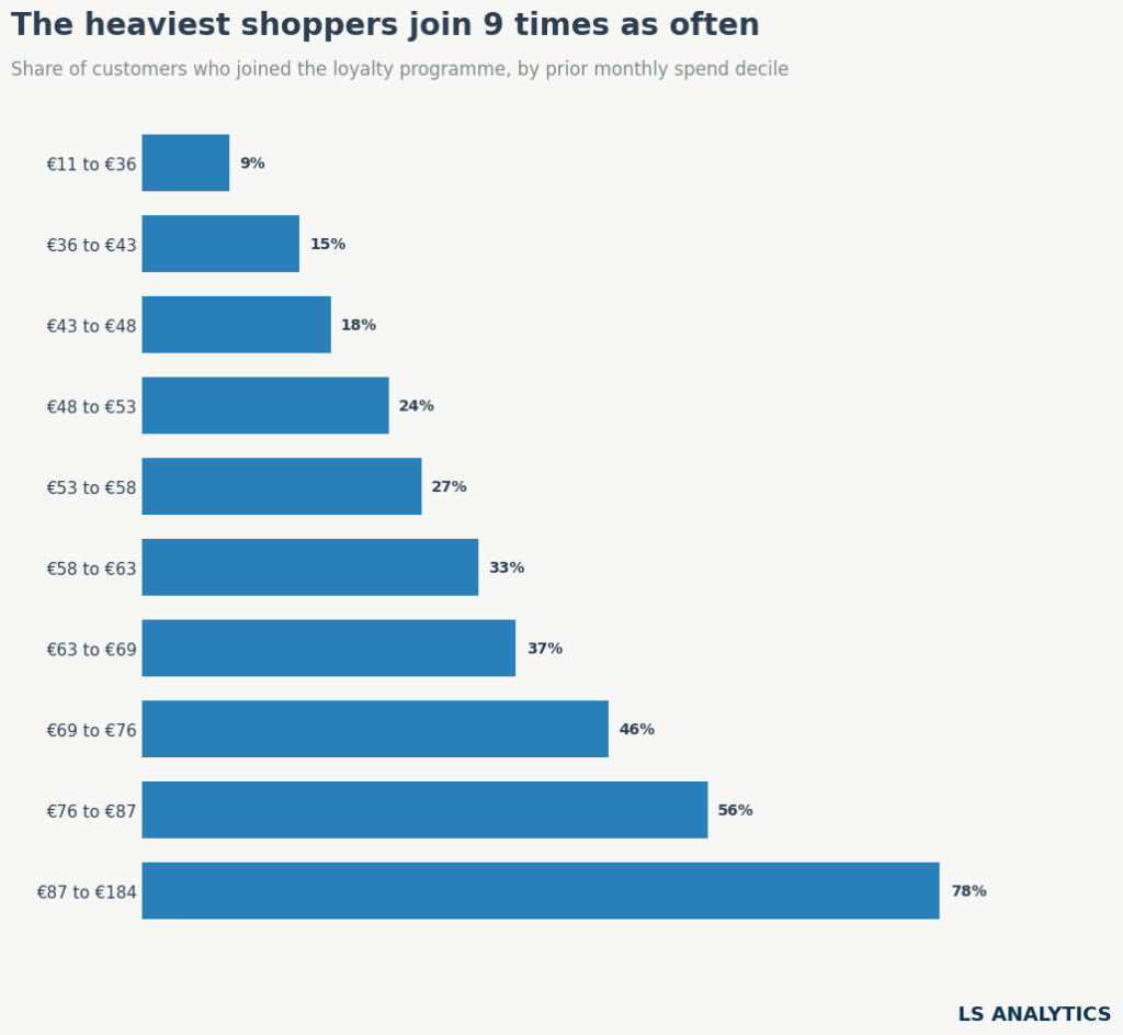
Spending habits are sticky, so a customer who spent €90 before the program launched was likely to be a high spender whether they joined the program or not. Following this logic, members would outspend non-members in every situation, even if the loyalty program did nothing. It doesn’t allow us to conclude the efficiency of this marketing activity by simply comparing the two groups.
Confounding: when one factor drives both sides
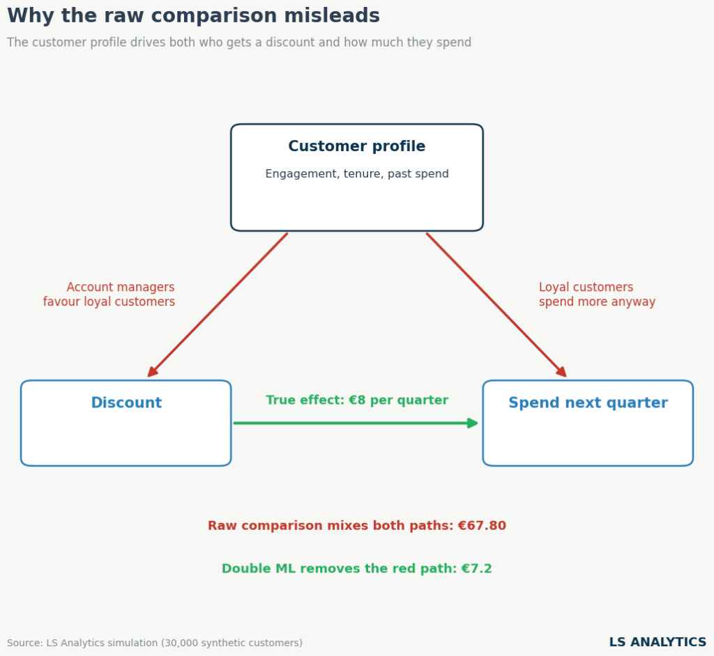
In causal inference terms, we call a variable like prior spending a confounder. It affects simultaneously the customer’s decision to join the program and their subsequent spending. When one factor drives both the treatment and the outcome, it opens a gap between groups even if the treatment has no effect.
A causal diagram is the best way to visualise such a situation. Each box is a variable, and arrows indicate which variable causes another.
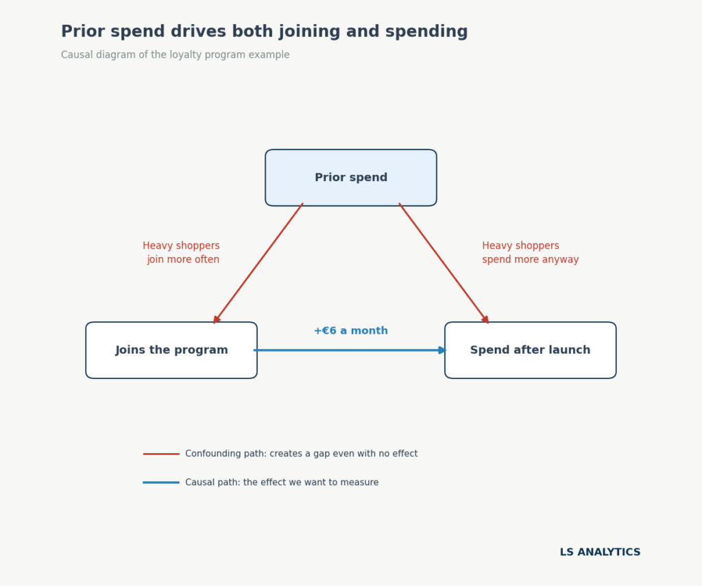
Two paths here connect the program to spend after launch. The blue arrow is the effect we are after: how much the loyalty program changed customers’ spending behaviour. However, the red path through prior spend complicates this: customers with higher prior spend are more likely to join the program and will also spend more after launch. The red path is called a backdoor path. Causal inference aims to block it so only the blue path remains.
The fundamental problem of causal inference
We can achieve this goal in many ways. But before we discuss them, we should focus on the fundamental problem of causal inference, because understanding it is essential to understanding causality.
In our example, each customer has two possible actions in the future, assuming we are just before launching the program. They can either join the program or not. Each action comes with its own outcome. Conceptually, we would compare each customer’s spend if they joined the programme with their spend if they didn’t. The difference between those two potential outcomes is the loyalty program’s causal effect on the customer’s spending.
This concept sounds easy, but it’s only theoretical. In practice, we can observe only one outcome for each customer: their spend under the choice they actually made. We don’t know what this particular customer would have done without joining the scheme. This is a fundamental problem in causal inference; estimating ways to overcome it is another way to think about causal problems.
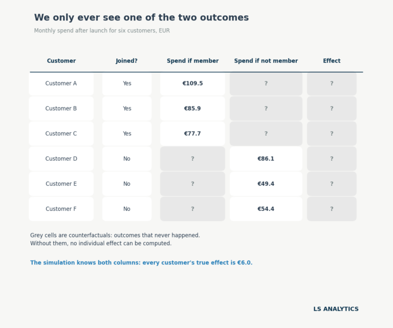
The following table highlights this issue. For everyone who joined the loyalty program, we know how much they spent after joining. For everyone who didn’t join the program, we know how much they spent without joining it. The question marks are the gaps we want to estimate from the data to understand the program’s true effect.
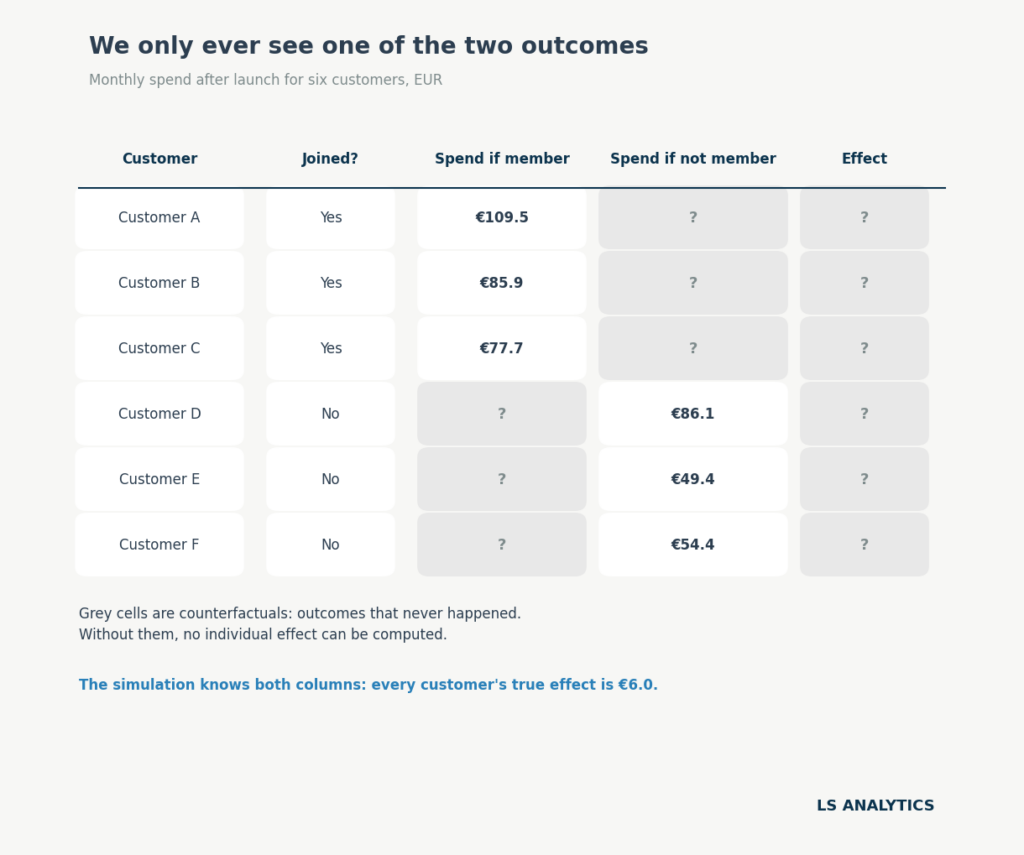
Grey cells in this table are called counterfactuals. A counterfactual is the outcome a unit would have had under the treatment it did not receive. In simpler terms, for customer A, the counterfactual is the spend this customer would have generated if they hadn’t joined the program. For customer E, it’s the opposite: the counterfactual is the spend they would have had if they had joined the program. Calculating all counterfactuals lets us estimate the program’s effect at both the individual and overall average levels. Usually, calculating the average treatment effect (ATE) for the group as a whole is easier. Still, more advanced methods can also estimate the so-called conditional average treatment effect (CATE), even at the single-unit level.
Estimating counterfactuals is treated differently in two main approaches towards causal inference. The potential outcomes framework, developed by Donald Rubin in the 1970s, assigns each unit one outcome for each possible treatment. A causal effect compares those outcomes.
A causal graph, associated with Judea Pearl and his causal calculus, starts from a diagram. We draw what causes what, and then we decide which variables to adjust for and which to leave alone. The confounding diagram earlier is a simple example of using graphs in causal inference.
In practice, both approaches complement each other. We can start by drawing a causal diagram to understand the problem’s structure, then use the potential outcomes framework to define the effect and choose an estimation method.
How causal inference works
Causal inference methods differ in their design and internal mechanics. However, most causal inference applications share a common workflow that can serve as a useful framework.
Step 1: Define the effect you want
Asking ‘Does it work’ or ‘Does the program work’ is slightly too vague and needs more precision. The precise causal question defines the population or group of interest and the outcome we want to measure. For example, we would like to know whether introducing the program incresed the spending of customers who joined it.
At this point, it is important to differentiate the two versions of the causal effect we can measure. This matters because different causal methods measure slightly different things.
To start with, we can measure the effect of the loyalty program on its members, which will answer the question How much more do members spend because they joined?’ The causal effect measured only for the population that received the treatment is called the average treatment effect on the treated (ATT).
On the other hand, we might want to quantify a more general effect. How much more would the average customer spend if enrolled on the program? This causal effect applies not only to customers who joined the program, but also to the overall population of interest. It is called the average treatment effect (ATE). It tells you what to expect if the program were offered to all customers.
The difference between ATT and ATE is subtle, but they can differ, so always be clear which one you are measuring. Heavy shoppers make up a bigger share of members than of customers overall. If they gain more from joining, the ATT will be larger than the ATE. In our simulation, every member gains exactly €6, so the two are equal. Real data rarely works out that neatly.
Step 2: Write down assumptions
The second step in this framework is to draw a causal graph, or DAG (directed acyclic graph). The one we drew before says that prior spend drives both joining and later spending, and nothing else does. That is a strong claim, and in reality, we should consider many more factors. Of course, at this level some generalisation is needed, as we can never include all possible factors influencing the outcome. But we must include the ones that most strongly influence both treatment and outcome. Leaving one out biases the estimate; the stronger the confounder, the bigger the bias.
The diagram cannot be proven from data, and it comes from domain knowledge and information about the specific problem at hand. Its value lies in making the assumptions explicit so that anyone can challenge and address them. It also tells us what to adjust for.
Step 3: Choose a design and estimate
With the effect defined and the assumptions written down, the next step is to pick a method from the causal inference toolkit. This choice depends largely on how units were assigned to the treatment.
Based on this, we can distinguish two broad families of causal inference approaches.
Experiments are the first of them. The treatment assignment is controlled and random. This means that every potential confounder is balanced between the control and treatment groups. When randomisation is possible, it is the strongest design for measuring causal effects.
Without randomised data, we have to rely on observational data. We don’t control who gets treated here, as other factors determine treatment. Some designs find variation that behaves like a coin flip, for example, a policy that started on a known date, an eligibility cutoff, or a factor that influenced treatment without influencing the outcome. Others compare treated and untreated units after adjusting for the confounders.
In the next section, we will match each situation to a specific method. In the loyalty program case, randomisation is obviously not possible, as customers choose whether to join the program. This means we have to rely on observational data to estimate the causal effect. Fortunately, this case is rather simple, as we measured only one confounder. In such cases, measuring the causal effect is straightforward: we adjust for the confounding variable.
And this is exactly what we are about to do. To start, we can divide the customer base into buckets defined by the prior spend. We split customers into ten bands, so each band holds customers with similar habits. Within a band, members and non-members started from the same place, so any remaining gap comes from the programme.
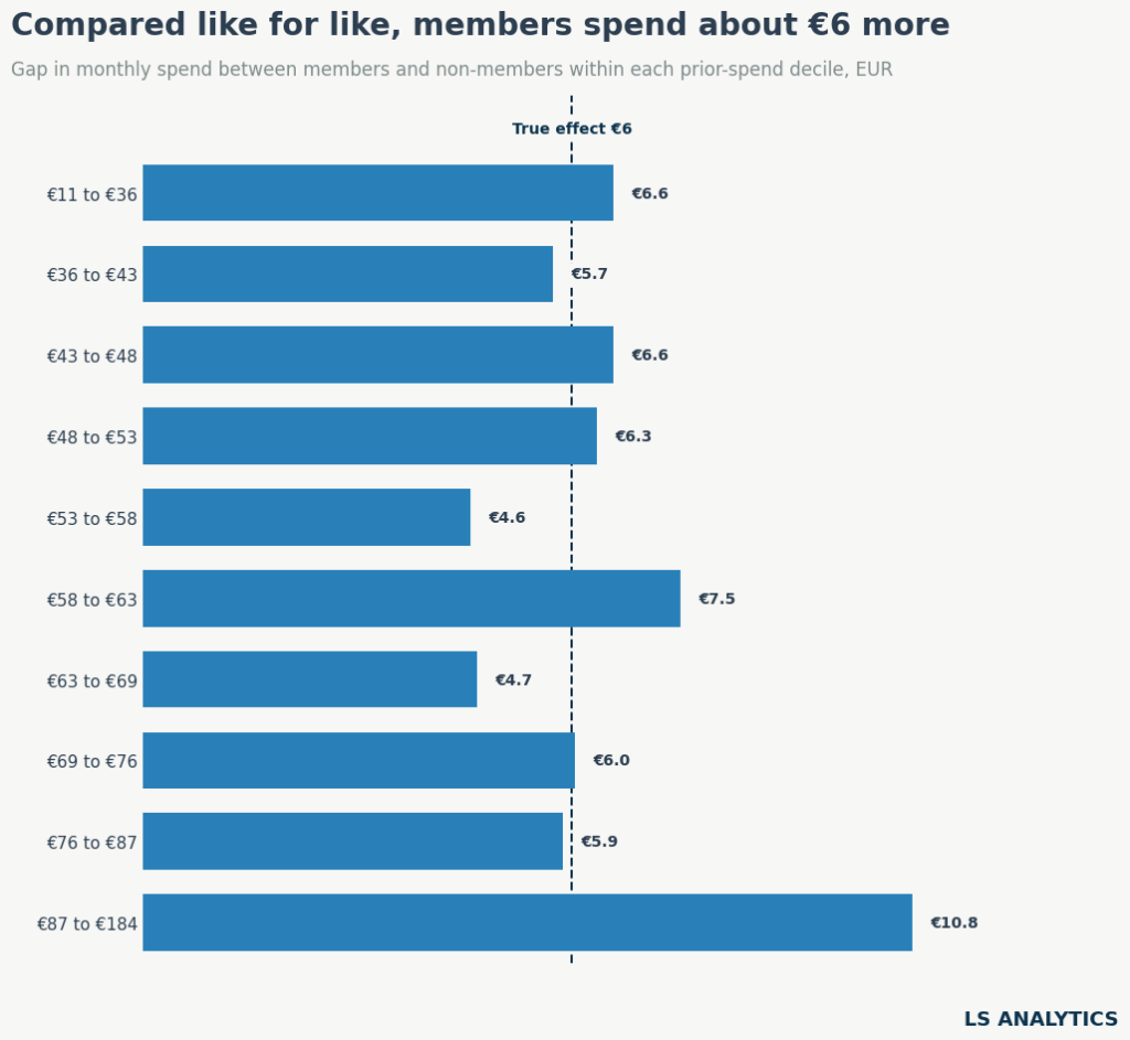
Nine of the ten bands show a gap between €4.60 and €7.50. Weighted by member count, the average is €7.00. The naive gap was €23.49.
The top band is the exception, at €10.80. It covers customers from €87 to €184 a month, a range too wide to cover many similar customers. Its members still spent more before launch than non-members, but this shows stratification works best with narrow bands.
We can fix this with a regression adjustment. It controls for prior spend as a continuous number and avoids splitting it into bands. The estimate is €5.80, with a 95% interval of €5.40 to €6.10, which contains the true treatment effect.
Main causal inference methods and when to use them
Many causal inference methods estimate the counterfactual and causal effect in different ways. The main ones include:
- Randomised experiment (A/B test). Considered the gold standard of causal inference. Treatment is assigned randomly, so the groups differ only by chance. The untreated group serves as a direct counterfactual.
- Difference-in-differences. Compares how an outcome changed over time in a treated group against an untreated one. The untreated group’s change shows what would have happened without the treatment. This holds only if both groups would have followed parallel trends without it.
- Synthetic control. Builds a doppelgänger for a single treated unit from a weighted mix of untreated units, such as other regions or stores. The gap between the unit and its synthetic version after launch is the effect.
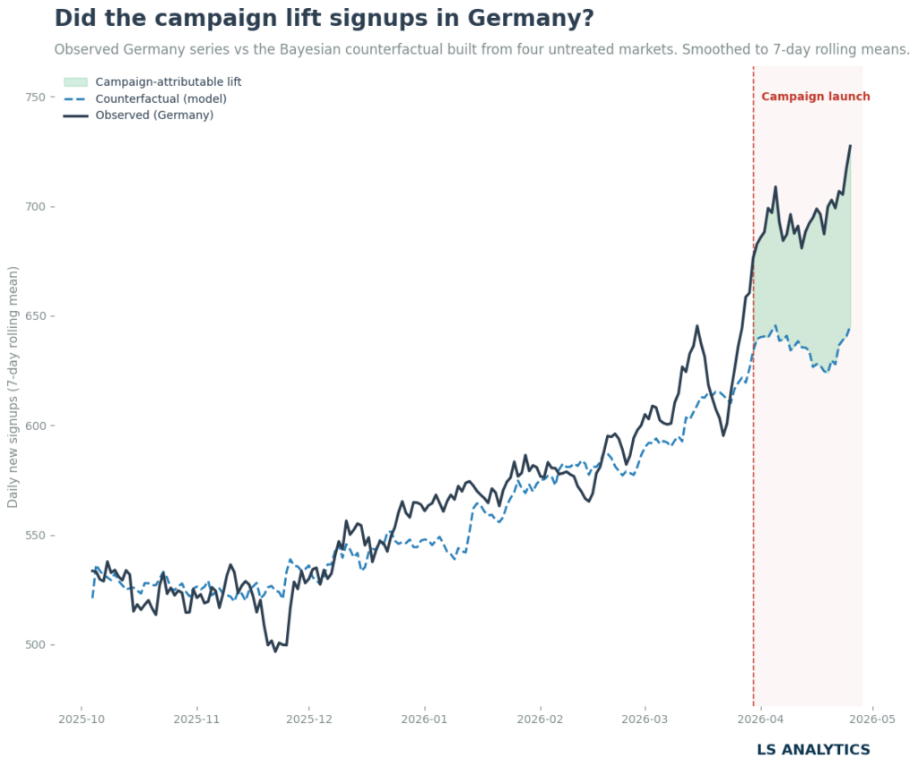
- CausalImpact. Fits a time-series model to the treated unit before launch, using untreated series as predictors. It forecasts what would have happened without treatment and compares that forecast with what did happen.
- Regression discontinuity. Compares units just above and just below a cutoff that decides treatment.
- Instrumental variables. Uses a factor that pushes some units into treatment and has no other path to the outcome
- Matching. Pairs each treated unit with one or more untreated units that look alike on measured traits, often summarised in a propensity score.
- Weighting. Assigns each unit a weight based on its likelihood of being treated. The weighted groups match on traits, and you can compare their outcomes directly.
- Regression adjustment. Models the outcome as a function of treatment and confounders. The treatment coefficient estimates the effect while holding the confounders fixed.
- Uplift modelling. Estimates how the effect varies from customer to customer. Each customer gets a score showing how much treatment changes their outcome. An uplift model predicts who will buy because of the treatment.
- Double machine learning. Uses flexible machine learning models to strip out the confounders’ influence from both treatment and outcome, then estimates the effect from what remains.
Choosing between them follows the logic from Step 3. Start from how treatment was assigned, and prefer the strongest design your situation allows. Often, it helps to imagine the perfect experiment, then, if it’s not possible, consider other approaches that best fit our data and problem at hand.
Causal inference assumptions you cannot skip
There are no free lunches, and causal inference is no exception. Every causal method relies on assumptions necessary to conduct the analysis correctly. Remembering them and stating them in each report is crucial and ensures not only a reality check for the causal analysis but also its .transparency
Some assumptions are method-specific, but a few core causal infernece assumptions apply across almost all causal studies.
No unmeasured confounders is the first, and likely the most important, of these. Here, our dataset must include every factor that drives treatment and outcome. Our estimate of €5.8 holds because prior spend is the only confounder, and we measured it and included it in the analysis. Imagine that heavy app users are more likely to join the loyalty program and spend more. But the company never tracked app usage, and it is not included in the data. Without this data, the final estimate will be biased because we can’t account for this confounder or its causal effect. We can measure the sensitivity of our estimate to unmeasured confounders, but we generally have to assume that no strong confounders are omitted.
Another assumption common in causal inference is overlap. To simplify, every group in the analysis should have both treated and non-treated units. For example, in our analysis, every customer type needs both members and non-members for comparison. In our data, even the heaviest spenders include some non-members: 78% joined, and 22% did not. If all of them had joined, the data would say nothing about what heavy spenders do without the programme.
It is also common to assume no spillover between units. Treatment effects from the treated units shouldn’t influence the behaviour of non-treated units, as it might change their activity. For example, one customer’s treatment should not change another customer’s outcome. In practice, this breaks down more often than we can expect. Members get early access to sales. If they clear the best stock, non-members find less to buy and spend less. That widens the gap and inflates the estimate.
And those assumptions often can’t really be tested. After all, we usually have access to only one dataset, and we can’t be sure what’s happening outside of it. Fortunately, sensitivity analysis can help. It asks how strong a hidden confounder would need to be to make the effect disappear. If only an implausibly strong one could, the result stands. If a modest one would change the results, we have to report the estimate with that caveat. Tools such as DoWhy’s library refutation tests help us check those assumptions.