The most important question in almost any organisation is also the hardest: Did something work?
You launch a new feature, a pricing change, or a new loyalty program. Your stakeholders want to know whether it worked.
The pressure to answer quickly is always immense. The fastest way to evaluate an action’s effect is to check whether a metric changed after implementation. To prove or dismiss the value of such actions, analysts often reach for the simplest tool in their arsenal: pre post analysis. You calculate the average performance before the action, do the same after it, and calculate the uplift.
It is intuitive. It is fast. And very often it is wrong.
Pre/Post Analysis relies on a single, simple, but very strong assumption. The world would have continued the same if we hadn’t performed a specific action. It assumes that, without intervention, our metrics might have remained unchanged. Hence, any change after the intervention is caused by it.
But the world is much more complex, and that statement requires strong certainty. After all, we have seasonality, competitors’ activity, and an almost immeasurable number of possible factors that can influence the environment.
As analysts, our job is to separate correlation from causation. In this article, we set aside intuition and use simulated data to explore how this trap works.
Simulating a loyalty program with zero true effect
Let’s start by building our simulation. To understand the Pre/Post trap, we first need to build a world where we know the truth. This way, we can easily see how it can be violated.
Imagine you are the Data Scientist at a growing e-commerce platform. The Product Team believes that the users aren’t spending enough, so they designed a new loyalty program for the most valuable customers. We will call the program ‘intervention’ to align with the causal inference terminology. The program launched on 1st October 2023 and aimed to increase average revenue per user.
In our simulation, we will assume the Almighty’s power and define the ground truth. We will set the program’s true impact to exactly zero. It didn’t help us improve our revenue at all.
We will also include the confounder: a hidden seasonal trend. As the end of the year and the holiday season approach, users start to spend more, regardless of the loyalty program.
Let’s simulate the data using the following code.
start_date = '2023-07-01'
end_date = '2023-12-31'
dates = pd.date_range(start=start_date, end=end_date, freq='D')
n_days = len(dates)
launch_date = pd.to_datetime('2023-10-01')

base_arpu = 15.0
noise = np.random.normal(0, 1.5, n_days)

day_of_year = dates.dayofyear
seasonal_trend = np.where(day_of_year > 245, (day_of_year - 245) * 0.08, 0)

true_intervention_effect = 0

daily_arpu = base_arpu + seasonal_trend + true_intervention_effect + noise
df = pd.DataFrame({'Date': dates, 'ARPU': daily_arpu})
The pre post analysis trap: a 38% uplift that wasn’t real
As the year ended, the Product Team approached us again and asked us to measure the loyalty program’s impact. The first and correct approach is to check the daily revenue generated by our shop’s users. We plot this and see the following.
Looking at the chart above, we clearly see the results any product manager would love. The average daily revenue from our shop users was 15 USD before the loyalty program launched. After the program started, it increased to 21 USD per day. It’s a massive 38% uplift. The math here is perfectly accurate.
If we put this slide in the deck summarising the quarter’s performance for an audience that isn’t composed of data specialists, we could get a lot of applause for showing strong traction. And the executives would likely approve the budget to keep the loyalty program.
But we have to take a step back. As data scientists, we know that understanding how we generate data and drive insights is the most important part of the job. And the chart above is a textbook example of the Pre/Post trap. We distilled the customer behaviour into two averages, hiding the context that matters most.
Why seasonality breaks pre post analysis
To understand why the analysis above is incorrect, we need to consider counterfactuals. It is a term from causal inference that effectively asks what would have happened otherwise.
We have to ask ourselves: What would have happened to our revenue if we had never launched the loyalty program?
And of course, this is a very difficult question, as we can never be sure about something that did not happen. Causal inference uses multiple methods to try to discover this. They even give Nobel Prizes for advances in this field.
Going back to our example. By conducting the Pre/Post analysis, we assumed that our counterfactual is the same as before. Specifically, we assume that without the loyalty program, average revenue per user would remain the same as before, around 15 USD. Therefore, we attribute any uplift after launch to the loyalty program.
It is not difficult to see how strong this assumption is. In all cases, we assume that past results would be the same in the future in the absence of measured action.
And we also know it is not true in our example. In the simulation, we introduced a seasonal trend. Spending naturally increases during the holiday shopping season in the last quarter of the year.
This is shown in the chart above. The seasonal trend shows that revenue started to increase just before the loyalty program launched. It started rising in September, and the loyalty program launch did not affect it.
Going further, we can see that the ‘post’ period coincided with the holiday season. The users were going to spend more money anyway. In reality, the new loyalty program did not contribute to the increase in customer revenue. The entire lift we observed was us taking credit for the holiday season.
This is why Pre/Post Analysis is dangerous. It blinds us to external factors (confounders) like seasonality, competitors’ activity, and economic trends. All those factors can influence our metrics of interest at the same time, making a simple comparison unreliable.
So, if we can’t trust the ‘Before vs After’ comparison, what are the alternatives?
The fix: run an A/B test
We need a method that captures the counterfactual. The approach that helps us answer what would have happened without the loyalty program. The best approach is to conduct a Randomised Controlled Trial (RCT) or an A/B Test, using whichever term is more business-oriented.
The basic logic to run is quite simple. And I’m simplifying here on purpose, as the design of the experiment can get way more complicated to avoid negative effects, like spillover. But let’s keep things simple to understand the logic.
Instead of launching the loyalty program to everyone, we randomly split our users into two groups. The treatment group will get access to the new program, and the control group won’t. We assume customers in the control group won’t know about the program.
Because both groups exist simultaneously, they are both exposed to the same external factors. And what’s more, due to random selection, they are comparable in all observable and unobservable characteristics. The only difference is that one group receives a loyalty program. For example, both groups will spend more during the holiday season, leading to higher spending.
By comparing the two groups, we automatically control for all confounders. Any difference in revenue between them will be solely due to the treatment.
Let’s simulate the results of such an A/B test on the chart below.
Running an experiment confirms what we observed in the section before. Here, the lines for the control and treatment groups move in the same direction after the loyalty program launches.
It shows that the program’s incremental impact is effectively zero. The A/B isolation separated the treatment from external noise. Running the test helps the company save money by avoiding the cost of investing millions in a program that doesn’t actually work.
When is pre post analysis acceptable?
After seeing those results, we might be tempted to ban the Pre/Post analysis entirely. But before we do it, let’s assess whether it can ever be useful and under what conditions. After all, there are many situations in which running an A/B test is impossible.
If we must use Pre/Post analysis, we must acknowledge the strong assumptions underlying it. There is no escape from it.
This analysis requires that the statistical properties of our metric of interest are constant in the world without the treatment. We assume that everything would have remained the same over time without intervention. We are basically betting that nothing else in the world has changed.
And we can already see how hard that is to achieve. To claim it, you need a thorough understanding of the problem.
And if we really don’t have a choice and have to make such a comparison, it’s always better to track changes over a shorter time frame. For example, comparing data at the daily or hourly level is much safer than at the monthly level. Fewer factors can change in a shorter time frame.
And the higher the probability, the more likely the event caused it. We can be much more certain that the technical error caused a 60% drop in website traffic than a 2% decrease. This is, of course, a rule of thumb, not a scientific or fixed approach.
And it’s always better to have some benchmarks to compare changes. For example, when we see the result of the change in the registration form in one region, it’s always good to compare the trends with those in other regions. Basically, anything that can reduce our uncertainty is useful. And in all cases when we are forced to run Pre/Post Analysis, we must always consider domain knowledge, experience, and sometimes a bit of common sense.
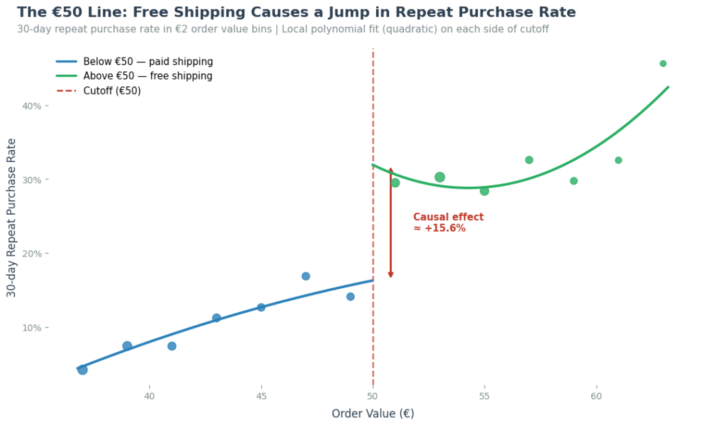
And not everything is lost, even if we can’t run an A/B Test easily. A large and very useful family of quasi-experimental methods includes difference-in-differences with a synthetic control group. They are designed to help us estimate causal effects even from observational data. This is a core part of causal inference, and it’s always preferable to use these tools instead of relying solely on Pre/Post Analysis, especially when the potential cost or benefit of discovering the true causal effect is large.
Timing is not causation
If our example shows one lesson, it is that timing is not causation. Just because two things happen at the same time, like the loyalty program and a spike in revenue, doesn’t mean that one caused the other. As we saw, a 38% lift can in reality be non-existent.
Analysts are often rushed to deliver results and showcase the effect of something. But it’s not what we are paid for. We are paid to deliver or be as close to the truth as possible. That’s why understanding the pitfalls of the Pre/Post Analysis is essential. It also shows why causal inference matters. It helps us discover the truth in a messy, complicated world.