When Amazon Prime launched in 2005, it changed delivery costs from a transaction cost into a membership benefit, something customers expect. Once customers experience it, paying for e-commerce delivery starts to feel like a step backwards. Competitors had little choice but to follow, offering various free delivery programs. Today, free shipping above a certain spend threshold is standard for most e-commerce shops.
What is often missing in evaluating such programs is a simple question: Did it really work?
Imagine a European retailer offering free delivery on all orders above 50 EUR. The aim of such a program is simple: to reward higher spending behaviour and drive customer loyalty. But introducing such a program raises a crucial strategic question. Does free shipping actually make customers come back and spend more? Or would customers have come back even without this feature?
This is a very important distinction. If free shipping drives retention, the program is valuable and could be expanded. If the opposite is true, the program becomes an expensive way to subsidise behaviour that would have happened anyway. Any profitable business wants marketing activities to drive incremental sales.
Answering this question correctly isn’t straightforward, because we have to measure a causal effect. We can’t answer it by looking at correlations alone.
This is the problem that causal inference exists to solve. When we can’t run randomised experiments, we have to look for the best possible solution. And we often find them in the so-called quasi-experiments.
The regression discontinuity design is one of them and is perfect for answering a question like the efficiency of the free delivery program. The models assume that access to a treatment (free shipping) is triggered once the threshold is reached. The basic assumption here is that customers above or below 50 EUR are quite similar.
After all, someone who spends 49 EUR is not much different from someone spending 51 EUR. But only the second person receives free shipping. A regression discontinuity design is an ideal method for examining how free shipping affects customer behaviour around this threshold. In this article, we walk through how it works, how to run it in Python, and how to test whether the results hold up under scrutiny.
RDD Intuition
The most obvious step to take when analysing the problem like this is to compare two groups of customers, those who used the free shipping and those who didn’t, and then to compare their repeat purchase rates. It’s quick and intuitive, but we should use it only as a starting point, since it can lead to misleading results.
The chart below shows what is clear. Customers who use free shipping make subsequent purchases at a much higher rate than those who don’t.
But we can’t just end there. In fact, customers who use free shipping must spend more. This makes them more valuable customers and, therefore, more likely to buy more products in the future.
This is visible when we break down the retention rate by spending brackets. Repeat purchase rates rise steadily with order value, even before we introduce free shipping. Customers who spend €80 return more than those who spend €60, who return more than those who spend €40.
This is not because of free shipping. It is because customers who spend more are more engaged, more loyal, and more affluent. The free shipping threshold falls in the middle of the trends, and based on this data, we cannot conclude whether the program had any incremental effect.
Fitting a simple regression model using the threshold as a treatment indicator won’t solve the problem either. The simple linear regression appears smooth, but it doesn’t capture the jump in repeat purchases around the free shipping threshold.
It attributes the entire relationship between order value and repeat purchase to a simple trend. This approach will not tell us whether the free shipping program has any causal effect on customer retention.
We need a method to isolate the effect of the threshold itself. We need to ask: Do customers who received free shipping return more? But does crossing the €50 line, and only that, change what a customer does next?
This is exactly what Regression Continuity Design does.
The only thing that differentiates those groups is an externally imposed rule. The difference around the threshold is not a customer quality issue. The company created it by setting a threshold during meetings. And RDD frameworks take advantage of such situations.
The logic of this method is quite simple. Customers around the threshold line should be quite similar. Those just above or just below the line should be essentially identical. This assumption is intuitive. After all, why is someone spending 49 EUR drastically different to someone spending 51 EUR? In such cases, the difference in value is negligible, but only customers who spend over 50 EUR are eligible for the free shipping program.
In the language of RDD, the order value is the running variable, the continuous measure that determines treatment. Customers above the 50 EUR threshold receive free shipping, and those below it do not. The outcome we care about is whether a customer makes a repeat purchase within 30 days.
If free shipping causally affects repeat purchases, we should see a specific pattern in the data: a sharp, discontinuous jump in the outcome at the €50 threshold.
Assumptions
All causal inference methods rely on a few assumptions that we must state before running them. It does not make causal inference less practical. On the contrary, they enhance our understanding of the method and its limitations and help us choose the tools we need to answer the question. The regression discontinuity design has three main assumptions we must make before applying it.
Continuity is the first of them. Technically, it states that in the absence of treatment, the expected potential outcomes would change continuously at the cutoff point. What does it mean? We have to assume that, without free shipping, there should be nothing special about the 50 EUR threshold. The relationship between order value and repeat purchase rate should follow a smooth curve, with any jump attributable solely to the treatment itself.
This assumption would be violated if something else had changed at the 50 EUR order value. For example, the retailer could trigger an email campaign with discounts for customers who spend about 50 EUR. In that case, any change in the outcome would be a combination of the free shipping effect and the email promotion. And we couldn’t separate those effects.
Unfortunately, we can’t directly test this assumption. We see only one world, and we cannot know what would have happened in its absence. After all, we wouldn’t need causal inference if we already had such information. But we can always look for evidence against this assumption based on our understanding of the problem. For example, we could check whether any other marketing activities trigger at exactly 50 EUR order value. If the answer is no, then the assumption is defensible. Testing this assumption requires not only checking the data but also understanding the problem. Discussing it with business owners is a great way to understand it and gain more domain knowledge, which is essential for most causal inference questions.
The second assumption we state is that there is no precise manipulation. We will contradict ourselves here, as in the section below, we will show that we might encounter this in the case of free shipping. This assumption states that customers cannot manipulate the threshold, meaning they cannot purposefully change their behaviour to place themselves just above or below the cutoff points. Violating this assumption makes the regression discontinuity analysis more difficult. But it depends on how the manipulation occurs. If everyone above or below the threshold is there by design, the analysis won’t be reliable because both groups would be fundamentally different.
The standard diagnostic tool for assessing this assumption is to plot the treatment variable and examine clustering around the cutoff. A smooth distribution with a modest jump is tolerable. A spike concentrated at a single value is a cause for concern. We will look at this directly in the next section.
The last assumption we will mention is not necessarily the one that will make or break the analysis, but rather a characteristic of this approach that shows what kind of treatment effect we can obtain from a regression discontinuity design. We must remember that we can estimate the effect only for customers near the threshold. RDD will never tell us what the impact of the free shipping program is for customers who spend, for example, 20 EUR. We will never find out using this method what will happen if we change the free shipping threshold from 20 EUR to 25 EUR. It can tell us only the effect of moving the 50 EUR order value for a customer whose order value is close to the cutoff.
This is called the Local Average Treatment Effect as opposed to the Average Treatment Effect. Local because we estimate it only locally, around the cutoff point. It’s not a limitation of this method. We just need to remember which questions RDD can answer. With this method applied properly, and provided the other assumptions hold, we can confidently estimate the effect of the free shipping program on customers with orders around 50 EUR. But we can’t generalise those findings to the entire customer base.
Manipulating the Threshold
Before we run the analysis, something unusual about this example is worth addressing. The free shipping threshold is not invisible to customers, and they can respond to it deliberately.
Anyone who shops online regularly has, of course, done so. You have 43 EUR in your basket, but after noticing free shipping starts at 50 EUR, you add something else just to close the gap and get free shipping.
In causal inference terms, it’s called the manipulation of the running variable. It means the distribution of order values near the €50 cutoff isn’t purely natural. Customer intent has shaped it. If customers are actively manipulating their way above the threshold, then the group just above 50 EUR is not just a random sample of customers. A part of the group noticed the threshold, wanted the benefit, and acted on it.
And it is clearly visible in the data. An unusual spike just above the free shipping threshold suggests customers deliberately increase their order value to qualify.
The power of the regression discontinuity design lies in a single assumption. That customers just above and just below the cutoff are essentially the same. The only difference is whether they receive treatment based on meeting the threshold.
Manipulation breaks this assumption. When customers exceed the threshold, both groups are no longer comparable. The customers who spent just above €50 are not a random sample of people who happened to spend a little more. They are a self-selected group who purposefully spent more to receive the free shipping benefit. They may be more price-sensitive, more deal-conscious, or simply shop more often. Any of these characteristics could independently influence their likelihood of returning. The RDD estimate can’t distinguish the effect of free shipping from the effect of being a customer whose basket value increases to qualify for free shipping.
That said, it’s important not to overreact and to stop this analysis completely. Real-world data is messy, and we rarely have access to data that meets all assumptions. And sometimes it is better to run an imperfect analysis than to do nothing. Of course, with all the limitations of such an approach in mind. And what’s more, the observed manipulation is not perfectly accurate.
Customers increase their basket value, but they rarely increase it by exactly enough to reach 50.01 EUR. Some of them will spend 53 EUR, some 56 EUR. In practice, customers above the threshold are a slightly selected group, but not all of them are artificially selected. The RDD estimate remains meaningful, but it applies specifically to engaged customers rather than the average shopper.
More importantly, customers responding to the threshold is itself commercially important information. It tells you the programme is visible, customers are paying attention to it, and it is already influencing basket value.
There is also a plausible argument that topping up a basket creates a stronger relationship with the order itself. A customer who has actively modified their basket to reach a threshold has more invested in that purchase. They have spent more time on the site, considered more products, and made a more deliberate decision. That kind of engagement may independently increase the likelihood of a positive post-purchase experience. And with it, the likelihood of returning.
This does not mean we should ignore the manipulation. It means we should interpret the results with nuance. The effect we measure with RDD in this context is the effect of free shipping on customers who were close to the threshold and aware of it, which is precisely the population whose behaviour a threshold decision would affect. For most retail strategy questions, that is still exactly the number you need.
Running the analysis
The first technical step in conducting a regression discontinuity analysis is to centre the running variable around the cutoff. This lets us assess each order against the interest threshold. The process is very simple. We just have to subtract 50 EUR from each observation. This way, a customer who spends 47 EUR becomes -3, and a customer who spends 55 EUR becomes +5.
Such transformations seem small, but they are crucial to the validity of the RDD method. This means that when we fit regression lines on each side of the cutoff, each line’s intercept corresponds exactly to the predicted outcome at the threshold. The difference between those two intercepts is the treatment effect we want. Thanks to centring, we can discover it without any additional calculation afterwards.
The next step is to model the relationship between order value and the repeat purchase rate. The simplest choice, as usual, is a linear relationship. This works when the underlying relationship around the threshold is approximately linear. But in practice, most human behaviour is rarely linear. As the chart above shows, the relationship between order value and repeat purchase behaviour does not follow a straight line. It rises quickly at low order values, then flattens out as customers reach higher spending levels. Forcing a linear relationship would oversimplify the analysis. For that reason, we can use the quadratic function as a second-degree polynomial. It will allow us to better fit the trend described in our data.
Before we run the regression model, we have one more decision to make. We have to choose the so-called bandwidth, the window of observations included in the analysis on each side of the cutoff point. It is one of the most important decisions in RDD settings. If we set this window too wide, we will start comparing customers who are quite different from each other, which contradicts the whole idea of regression discontinuity. On the other hand, if the bandwidth is too narrow, we will have too few observations, making the analysis unstable.
As usual in the world of causal inference, there is no one correct and definitive answer on how to set this value. The intuition behind bandwidth selection is to keep it wide enough to provide sufficient data for comparison and narrow enough to keep customers on both sides comparable. Since there is no simple answer, methods can help us choose the optimal bandwidth. We can mention here the Imbens-Kalyanaraman (IK) Method or the Calonico-Cattaneo-Farrell (CCT) Method. Another approach is sensitivity testing: choose different bandwidths, run the analysis multiple times, and check how the estimate changes with different bandwidth values.
For simplicity, we won’t dig deep into the technicalities of different bandwidth calculation approaches. We applied the CCT method from the rdrobust library to find the optimal width of this range. We can do it by running the following Python commands:
from rdrobust import rdbwselect, rdrobust

bw_sel = rdbwselect(y=df.repeat, x=df.centered, c=0, p=2,
                     kernel='triangular', bwselect='mserd')
BW = float(bw_sel.bws.iloc[0, 0])

print(f"CCT-optimal bandwidth: ±€{BW:.1f}")
The algorithm returns an optimal bandwidth of 13.2, which we can now apply to the rest of the analysis.
At this point, we can run the regression models. More precisely, we need to run two models, one on each side of the threshold within the bandwidth. Before we do this, we can try to understand why we are running multiple models. After all, it might seem quite natural to run a single regression model with a treatment dummy variable.
But that approach might be dangerous, as the data above and below the cutoff points differ and come from two distinct data-generating processes. Running a single model would force a single curve to fit the different relationships between order value and repeat purchase rate. We assume that below the 50 EUR threshold, the relationship between those two variables is natural. It doesn’t include the free shipping effect. Above the threshold, we also observe a naturally increasing repeat purchase rate with order value, but modified by the free shipping effect. And it alters the relationship between purchase value and future shopping behaviour compared with customers below the threshold. To check whether such a free-shipping effect exists, we need to run two models.
Each independent model will describe the relationship between the variables of interest without being pulled by the other. Neither model will incorporate information from the other. This lets the relationship differ on either side of the threshold. If the repeat purchase rate increased faster at order values just below the cutoff, we could detect it. The single model would just average this effect.
And what’s even more important, running two models gives us the opportunity to discover the local causal effect. The gap between the two models is exactly the treatment effect we want to estimate.
This is the main mechanism of the regression discontinuity design. This model is not used to estimate the relationship between order value and retention. We are interested in identifying two local relationships and the discontinuity between them.
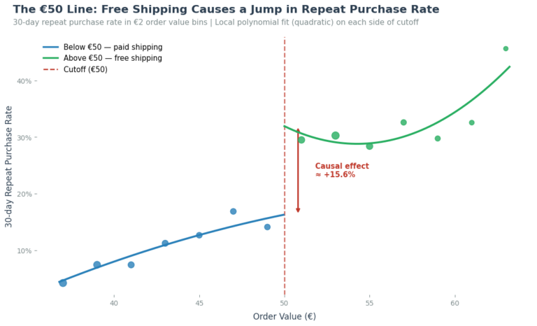
When we plot the data using those two curves, we can already see the first evidence of the positive causal effect of the free shipping program. A clear discontinuity appears around the order value threshold. We can also see that the relationship between order value and repeat purchase rate differs below and above the cutoff.
Each curve on the chart above predicts the repeat purchase rate under separate circumstances. The blue line shows the repeat purchase rate without free shipping. The green line shows the free shipping line. The vertical line gap at the 50 EUR order value shows the discontinuity and the local treatment effect.
Running two separate regressions provides a useful visual representation, but it’s not the optimal analytical approach because it doesn’t provide confidence intervals and p-values, which are important for assessing the validity of the discovered gap. Fortunately, there is an easy way to overcome this. We can run a mathematically equivalent model using a single regression formula. It uses interaction terms between the treatment indicator and the centred order value.
model_rdd = smf.ols(
    'repeat ~ centered + I(centered**2) + treatment'
    '       + centered:treatment + I(centered**2):treatment',
    data=df[df.centered.abs() <= BW]
).fit()
The formula looks complex, but it’s relatively straightforward once unpacked. It basically says: regress repeat purchase on the centred order value, its square, a treatment dummy indicator, and interactions between the treatment dummy and both polynomial terms. The interactions do the work of two separate curves in a single model.
Thanks to the addition of interactions, each curve on the left and right sides of the cutoff can have its own slope, exactly as in two separate regressions. Another advantage is that the treatment coefficient directly represents the treatment effect.
effect = model_rdd.params['treatment']
ci_lo  = model_rdd.conf_int().loc['treatment', 0]
ci_hi  = model_rdd.conf_int().loc['treatment', 1]
pval   = model_rdd.pvalues['treatment']
print(f"Estimate :  +{effect:.1%}")
print(f"95% CI   :  [+{ci_lo:.1%}, +{ci_hi:.1%}]")
print(f"p-value  :  {pval:.4f}")
This returns the treatment effect and its confidence interval.
Estimate :  +15.6%
95% CI   :  [+8.0%, +23.3%]
p-value  :  0.0001
Based on this, free shipping increases the probability of a 30-day repeat purchase by an estimated 15.6 percentage points for customers near the €50 threshold, with a 95% confidence interval of [8.0pp, 23.3pp]. The effect is clearly positive and statistically significant.
We could argue that the treatment effect may be inflated because customers are using free shipping to increase their order value. This could be true, and we should keep this in mind when running the analysis. This example was chosen specifically to showcase the difficulties of conducting causal inference in real life. Nevertheless, such a strong effect clearly indicates a positive impact of free shipping, even if it is smaller in practice.
Testing the Outcome: Placebo Test
So far, we have an estimate of the treatment effect and its confidence interval. Those numbers, nevertheless, are insufficient to determine whether they represent the true effect. The real question is whether these numbers reflect a causal effect rather than just noise. Good causal inference work does not stop at the estimate, but it actively tries to break it.
The standard way to do this is to conduct a placebo test. The logic of it is relatively simple. If the jump we observed at the 50 EUR cutoff was a true causal effect, then there should be no comparable jump at any other order value. The treatment effect should appear only at the actual cutoff point. Repeating the same analysis with a fake cutoff should yield a nonexistent treatment effect and non-significant results. However, running many such tests independently will produce false positives by chance.
For this reason, a good approach to running a placebo test is to use a stacked regression that evaluates each cutoff point. Basically, we have to stack our data into a single dataset, with copies for each cutoff value we want to test. Each cutoff value gets its own data with a chosen bandwidth window. In essence, each cutoff point has its own RDD model within the larger model to estimate the fixed effects at that point. This approach also enables us to run the joint F-test to assess whether all the fake cutoff points are jointly insignificant.
The chart shows the estimated effect for each candidate cutoff, along with the confidence interval. We can immediately see that all placebo cutoff effects are smaller than the 50 EUR threshold. Only the 65 EUR cutoff shows a slightly higher effect.
However, we also have confidence interval data. All the fake cutoffs show confidence intervals that contain zero. This means we can conclude that the RDD effects at each of those cutoffs are not significant. Moreover, the only confidence interval that does not include zero is the one for the actual cutoff we used in the analysis. It is very strong evidence for our causal claim.
Alongside the visual, the stacked regression delivers the joint F-test:
Joint F-test: placebos = 0
F = 0.17,  p = 0.991
The results are clear. The F-test asks whether the joint effect of placebo cutoffs is zero. A high p-value indicates that we cannot reject the null hypothesis, further validating the causal effect of free shipping. Only the real 50 EUR order-value threshold produces a discontinuity, which helps validate our analysis.
We have to remember that even a successful placebo test is not definitive proof of causality. No statistical procedure can deliver that on its own. It provides the strongest form of evidence available from observational data. It makes our case for the real causal effect of the 50 EUR free shipping cutoff on the retention rate substantially harder to dismiss.
Local Treatment Effect
At this point, we obtained a clear, defensible causal effect using the regression discontinuity design. One thing left to clarify is what we are actually measuring using the approach. We discussed this briefly when covering assumptions, but it is essential to understanding RDD and worth repeating.
The estimated results indicate that crossing the 50 EUR order value threshold and entering the free shipping threshold increase the probability of a repeat purchase by approximately 15%. This effect is substantial, but we have to be careful with interpreting it.
Does it mean that if we offered free shipping to all customers, regardless of order value, the probability of a repeat purchase would increase for everyone? It does not, and this is one of the most common misconceptions about regression discontinuity design. The estimate we recovered is called the Local Treatment Effect (LATE). And the ‘local’ part is the most important element of its name.
The effect we measured is the effect of the free shipping for customers whose order value is close to 50 EUR, not for the entire customer base. It is not the effect of removing the free shipping program entirely or rolling it out to all customers. The measured results show the impact of crossing the 50 EUR order threshold for customers who were close to it to begin with.
This distinction matters because it’s tempting to generalise the causal claim and claim its universality. But RDD works differently. The obtained causal claim is narrower in its nature. We computed similarity among customers by comparing those near the threshold. Since the method, in essence, is based on comparing this group, we have to limit the causal claim to this group as well.
The location of the RDD estimate doesn’t mean it’s wrong or impractical. We only have to interpret it carefully and consider the practical implications. In the e-commerce case, applying RDD is reasonable as it answers the question we need. This is especially true if we want to adjust the thresholds while keeping them close to the current ones. For example, if the marketing team wanted to raise the free shipping limit from 50 EUR to 45 EUR, RDD would give us exactly what we need. They are roughly similar to the affected population, so we can reasonably expect the causal effect to be similar. Not necessarily the same, and this assumption might not hold if external circumstances change, but it’s the logical consequence of the RDD model.
On the other hand, if the question we asked were whether we should extend free shipping to the entire population, then using the regression discontinuity effect would be misleading. This is a different question, and it requires different causal inference methods. RDD answered the question it was designed to answer: what the threshold, as it currently exists, does.
Summary
The deeper point of this article is not only explaining the regression discontinuity design in the context of e-commerce, but also distinguishing correlation from causation and how we can close that gap. Most data analytics still operate on correlations rather than causal inference. This is especially evident when A/B testing data is unavailable. Many business decisions are made based on purely correlational data without considering the causal structure.
Causal inference methods, like regression discontinuity design, do not give us a free lunch. We still need our data to have a certain structure, which is not always easy to find. Those methods require many assumptions that we have to be ready to defend. But when those conditions hold, causal inference can yield a more accurate estimate of the true causal effect than any approach based solely on correlation.
The key to unlocking the power of causal inference is to look for natural experiments wherever possible. And once we start seeing the business this way, the analytical possibilities open up considerably.