Every statistics handbook covers confidence intervals. And everyone who has ever studied statistics has been confused by the fact that confidence intervals do not equal probability. 95% confidence interval doesn’t mean that there is a 95% probability that a value lies within this interval. Many students of statistics struggle to understand this intuitively.
This is not an issue of not being smart enough to get it, but rather of the non-intuitive, yet still useful, definitions of frequentist statistical tools. Bayesian statistics, however, uses a different tool: credible intervals, which define intervals as probability statements about the parameter. It is less well known but still useful, and we will explore the differences between the two intervals.
Consider the following result from a conversion rate uplift A/B test:
95% confidence interval on the conversion lift: [−0.84%, +10.80%]
95% credible interval on the conversion lift: [−0.86%, +10.65%]
Both intervals cover almost the same range; however, their interpretations differ completely. The frequentist interval says “this procedure, repeated across many experiments, would contain the true lift 95% of the time”. It describes the method’s long-run behaviour. The credible interval says, “Given the data we observed, there is a 95% probability the true lift lies in this range”.
In the following article, wewill explain what both intervals mean, how to calculate them, and the implications of using one versus the other.
Confidence Interval vs Credible Interval: What Each One Claims
The difference between a confidence interval and a credible interval isn’t a matter of taste. It comes from different assumptions and construction techniques.
In the frequentist view, conversion lift is treated as a fixed but unknown number. We don’t know it, but we assume it exists. The data we use to estimate this value are random. Since the data is random, the confidence interval we calculate from it is also random. If we run the experiment again, with a fresh sample, we might obtain different data and a different interval. The 95% confidence interval is a statement about a technique used to obtain it. The 95% refers to how often that procedure, applied across many hypothetical repetitions, produces an interval containing the true value. Any single interval either contains the true value or it doesn’t.
The Bayesian view is different, and the role flips. This time, we treat the data as fixed since we have already observed them. We treat the parameter we want to estimate as uncertain and assign it a probability distribution. The credible interval is a statement about this distribution. Given the prior knowledge and observed data, what is the probability that the conversion lift falls in this range? It is a statement about a parameter conditioned on everything we know.
We won’t resolve the debate over which method is better, as it is not only scientific but also slightly philosophical. What we do, however, is try to understand the results from both approaches and see that, in many cases, they can be similar, although interpreted differently.
In the frequentist world, we treat our interval as ‘given’ because it’s a statement about the approach, not about the state of reality. The difference is subtle, but it returns in the most challenging interpretation. In the Bayesian world, the results are conditional on the data and priors. The final statement is easier to understand, but it is only as good as the data and prior knowledge we feed it. This means neither approach is perfect.
What a 95% Confidence Interval Means: A Coverage Simulation
The frequentist definition is easy to state and hard to interpret and picture. If we run the same experiment many times and build a confidence interval each time, then 95% of those intervals will contain the true value. But nobody thinks like that. We never run the same experiment many times to check this. We rarely (and sometimes regretfully) run the same experiment more than once.
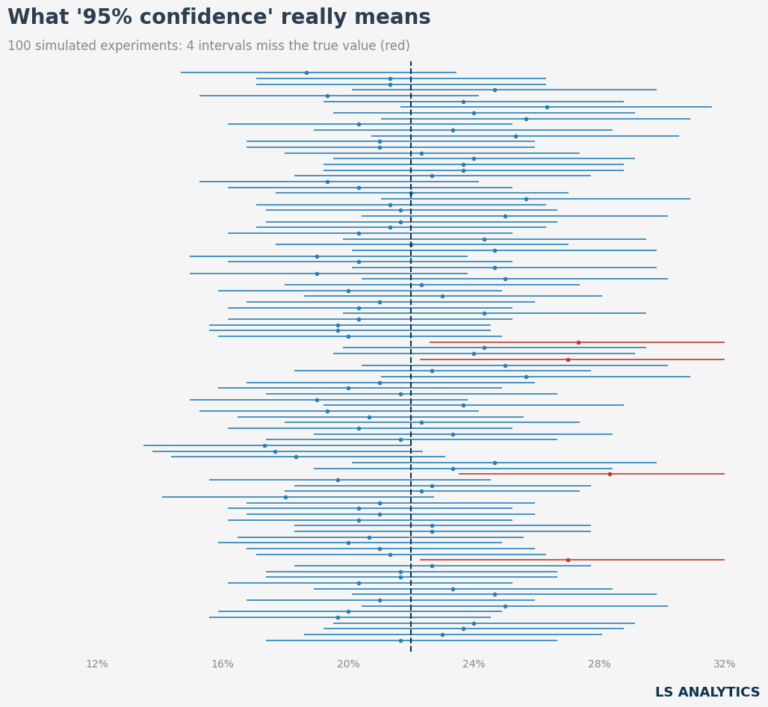
Let’s make this claim more concrete so we can better understand the confidence interval. We will do it by running a simple simulation. It draws 100 separate experiments from a known true conversion rate of 22%, each with 300 users. Since we fix the true rate by construction, we can check for each experiment whether its 95% interval captured it.
p_true = 0.22
n_per_experiment = 300
n_experiments = 100

sim = []
for i in range(n_experiments):
    successes = rng.binomial(n_per_experiment, p_true)
    lo, hi = proportion_confint(successes, n_per_experiment, alpha=0.05, method="wilson")
    sim.append({
        "experiment": i,
        "p_hat": successes / n_per_experiment,
        "low": lo, "high": hi,
        "covers": (lo <= p_true) & (p_true <= hi),
    })

sim_df = pd.DataFrame(sim)
Out of 100 simulated experiments, 96 of the intervals captured the true 22% rate.
That’s what 95% coverage means: not that any one interval has a 95% chance of being right, but that the method, applied over and over, gets it wrong about one time in twenty. And if we run more simulations, the results would converge to be even closer to the actual 95%.
A/B Test Example: Checkout Redesign, 400 Users per Group
The simulation above showed how theory works. Now it’s time to show the scenario analysts face in real life. We will have only one experiment, one dataset, and no way to observe the actual results. We need to apply statistical inference to understand the results.
Let’s use an example: a subscription paywall test. An e-commerce company’s product team redesigned the checkout flow and wants to know whether it converts better than the current version. Both groups ran for the same period with similar audiences.
The test had a control group and a target group, both with an equal number of customers. The control group had 82 conversions out of 400 users (20.5%), and the treatment group noted 102 conversions out of 400 users (25.5%). We also know that previous paywall tests at this company produced only small uplifts, rarely more than a few percentage points. This information will be very important when we start using Bayesian inference.
Both groups have exactly 400 users, so the split matches the plan. Real tests are rarely this tidy. When the counts drift further from the planned split than chance allows, you can’t trust the result, however clean the interval looks. That problem is called sample ratio mismatch, and it is worth checking before reading any A/B test result.
We chose 400 users as a deliberately small sample size to see what approaches work in a smaller-sample setup. Let’s code the test parameters by hardcoding the sample sizes and the number of conversions in both groups.
n_c, x_c = 400, 82   # control group
n_t, x_t = 400, 102  # treatment group
The observed lift is 5 percentage points. On its face, that looks like a clear win. Whether it actually is one, and how confident we can be, depends on factors such as sample size and variability. In this section, we will explore how to assess the significance of those results using both frequentist and Bayesian approaches.
Calculating the Confidence Interval in Python
Let’s start by calculating the confidence interval using the traditional, frequentist approach. We will use the following code to build it.
from statsmodels.stats.proportion import proportion_confint, confint_proportions_2indep

c_lo, c_hi = proportion_confint(x_c, n_c, alpha=0.05, method="wilson")
t_lo, t_hi = proportion_confint(x_t, n_t, alpha=0.05, method="wilson")
d_lo, d_hi = confint_proportions_2indep(
    x_t, n_t, x_c, n_c, method="newcomb", compare="diff"
)

print(f"CI control:   [{c_lo:.3%}, {c_hi:.3%}]")
print(f"CI treatment: [{t_lo:.3%}, {t_hi:.3%}]")
print(f"CI lift:    [{d_lo:+.2%}, {d_hi:+.2%}]")
The output of the code is as follows:
CI control:   [16.833%, 24.728%]
CI treatment: [21.476%, 29.990%]
CI lift:    [-0.84%, +10.80%]
What does it tell us? The intervals for the treatment and control groups overlap, suggesting the results are not statistically significant in the frequentist sense. This is confirmed by the confidence interval on the lift, which contains 0. At the 95% confidence level, we can’t be satisfied with the results and conclude that they’re unlikely to have been obtained by chance.
Let’s underline again what this interval actually tells us. It says that if we reran this experiment many times and computed this interval each time, about 95% of those intervals would contain the true lift. It doesn’t mean there is a 95% probability that the true lift lies between -0.84% and 10.8%.
And it also doesn’t tell us how likely it is that the modification in the checkout flow is actually bringing a positive value. We only know that we cannot rule out that those results were obtained solely by chance. It’s already an important hint, but we can try using Bayesian inference to see how it tackles the problem at hand.
Calculating the Credible Interval With a Beta Prior
The Bayesian version starts with a different question. It does not ask what range of values is compatible with the observed data. It asks what we should now believe about the lift, given both data and whatever we believed before running the test.
Incorporation of prior beliefs is the most controversial and disputed part of Bayesian inference. To calculate the credible interval, we have to state what we believe about the range of possible values before observing the data.
The whole framework is built upon this requirement. The prior is what we believed before seeing the data. Using this and the data, we obtain the posterior. The whole Bayesian framework shows us how to get from one to the other. What’s important is that both are distributions rather than single numbers. This helps us understand the range of plausible values and handle uncertainty better.
The objection to priors is obvious. Some of the results depend on something subjective. A prior is treated like a belief, and we update it. The stronger the evidence, the more likely the observed data will outweigh prior beliefs. But still, for Bayesian statistics to work, there is no way around including priors.
However, every action includes some pre-existing beliefs. Every experiment carries expectations about its results based on what we’ve observed before. We have information about the results of previous tests, and it anchors our beliefs about the new one. If most finished with conversion in the range of 20%, it would be unreasonable to believe the new one would end up at 2% or 80%. Bayesian inference insists we write it down rather than leave it. And when it’s stated clearly, we can always argue and challenge it. It’s no more subjective than how the world works in practice.
To start, we need a distribution to serve as a prior for the conversion rate. It has to cover values from 0 to 1 to align with the logic of conversion rate. The Beta distribution does exactly this. It takes two parameters, alpha and beta. The useful intuition is that alpha behaves like a count of prior successes and beta like a count of prior failures. A Beta(2, 8) prior amounts to saying “imagine I had already watched 10 users, and 2 of them converted.” That puts the centre at 20%, matching what past paywall tests showed, with the weight of exactly ten observations behind it.
Choosing the sample size of 10 is a deliberate option. Using a Beta distribution with the same probability of success but more observations would make a difference here. Since we are not entirely sure about the validity of prior tests and their importance for the new one, we used a weak prior. A weak prior nudges the results, but doesn’t steer them.
Had we picked Beta(20, 80), the same 20% would carry the weight of 100 observations and would visibly pull the result toward it. Generally, the larger the sample size in the prior distribution, the more weight it has on the overall analysis. We should use a strong prior only if we are sure about it and want it to dominate the analysis. Here, we want it to nudge the results, but still the observed data should do most of the work. That’s exactly what a weak prior is for.
Getting from a prior to a posterior is where the most important part of the Bayesian analysis happens. For the binomial data, we can use a property called conjugacy. We will omit the technical details here, but updating the prior distribution based on observed data is a simple addition. We take the prior’s observed successes and failures, combine them with the observed ones, and get the beta posterior distribution. The control group saw 82 conversions and 318 non-conversions, so its posterior is Beta(2 + 82, 8 + 318), or Beta(84, 326). And the same logic applies to the treatment group.
alpha_prior, beta_prior = 2, 8

post_c = (alpha_prior + x_c, beta_prior + n_c - x_c)
post_t = (alpha_prior + x_t, beta_prior + n_t - x_t)

print(f"Control  posterior: Beta{post_c}  mean {post_c[0]/sum(post_c):.3%}")
print(f"Treatment posterior: Beta{post_t}  mean {post_t[0]/sum(post_t):.3%}")
We now have two posterior distributions, each describing how plausible every possible conversion rate is given the observed data. But we need to calculate the lift of the test, which is the difference between the control-group and treatment-group distributions. Unlike the posterior distributions, there is no closed-form, analytical solution to obtain this number in a single equation. In such cases, the best solution is to run a simulation. We will draw values from both posterior distributions, subtract them, and store the result. The resulting structure is the posterior on the lift. We will prepare it using the following code.
n_draws = 200000
draws_c = rng.beta(post_c[0], post_c[1], size=n_draws)
draws_t = rng.beta(post_t[0], post_t[1], size=n_draws)
lift_draws = draws_t - draws_c

cred_lo, cred_hi = np.quantile(lift_draws, [0.025, 0.975])

print(f"Credible 95% interval for lift: [{cred_lo:+.2%}, {cred_hi:+.2%}]")
Credible 95% interval for lift: [-0.88%, +10.62%]
The results are surprising, as the obtained interval is almost the same as the confidence interval observed before. This was the outcome we wanted to show first, as we can see that with a small sample size and a weak prior, the two frameworks produce very similar arithmetic.
What separates them is that the credible interval is a probability statement about the lift. There is a 95% probability the true lift falls between −0.86% and +10.65%. We can use this intuitive statement freely, which is not possible with the frequentist approach. And once we have a full probability distribution over the lift rather than a single range, we can ask considerably more interesting questions than whether it happens to contain zero.
Questions Only the Posterior Can Answer
Both intervals give us almost the same range. Both include zero, and according to the frequentist approach, the results don’t allow us to conclude that the product change had any effect. But if a credible interval only restated the same range with different reasoning, there wouldn’t be much practical value in choosing between them.
The interval, though, isn’t what we build in the last step. We build a distribution over any possible value an experiment lift can have. The 95% credible interval summarises it by selecting the values that mark the middle 95% of this distribution. However, 95% is rather a convention than a final number we always have to follow. After all, why 95%, not 94% or 93%? The real value of the Bayesian approach lies in having access to the distribution itself. The same logic scales up. CausalImpact builds a Bayesian posterior over a counterfactual time series, so you get probability statements about campaign lift rather than a single point estimate.
Such a distribution is extremely helpful in guiding business decisions. The grey zone marks the region where the lift is negative, showing how likely the experiment is to be harmful. 4.8% of the posterior distribution falls there, leaving over 95% on the positive side.
We can ask direct questions about the distribution by checking the data directly. In the following code, we check the probability that lift is greater than 0, greater than 2, and greater than 5.
p_positive = (lift_draws > 0).mean()
p_gt_2pp   = (lift_draws > 0.02).mean()
p_gt_5pp   = (lift_draws > 0.05).mean()

print(f"P(lift > 0):     {p_positive:.1%}")
print(f"P(lift > 2 pp):  {p_gt_2pp:.1%}")
print(f"P(lift > 5 pp):  {p_gt_5pp:.1%}")
P(lift > 0):     95.0%
P(lift > 2 pp):  83.2%
P(lift > 5 pp):  47.4%
This procedure is easy and helps us better understand the results and quantify risk in more detail.
As mentioned above, we can see that there’s over a 95% chance that the experiment had a positive effect. At 83%, lift reaches 2 percentage points, and the probability of having lift higher than 5 percentage points is 47%. Whether those numbers give us enough confidence to say that the experiment had an effect is, in reality, a judgement call. We have to decide if a 95% chance of a positive effect is high enough. But this decision is not much different, and not much less subjective, than choosing a confidence interval in the frequentist world.
The two intervals described above gave us almost the same results, but they can still be used to answer the business questions we asked in different ways. It’s time to consider their advantages and disadvantages, as there is no clear winner that should be used all the time, and the application of either Bayesian or frequentist approach is often a matter of personal preference.
Which Interval Should You Use?
The Bayesian advantage is mostly about what we can say at the end. A posterior distribution gives us probabilities about the effect itself, which is an intuitive way to answer the business question. The frequentist approach requires more complex explanations. Applying prior knowledge is also a benefit, as it lets us use previously acquired information instead of starting each experiment from scratch.
The Bayesian approach can also be considered simpler, as it doesn’t involve alpha and beta, which are error probabilities in the frequentist approach. Understanding them has always been tricky in statistics, and we don’t have to worry about this when applying Bayesian intervals.
The cost of the Bayesian approach comes with applying the prior. Someone has to choose it, and this choice affects the final answer. Anyone reviewing the analysis might ask why we chose a particular prior, and this choice will always be disputable. The subjectivity of Bayesian statistics is a topic of much philosophical discussion, and we won’t solve it here; we should remember that it can also be a disadvantage.
Another drawback of the Bayesian approach is its higher computational cost. More complex Bayesian models require simulations, and fitting them can take significant time and resources. The frequentist approach is much faster, which helps when applying tests at scale.
The frequentist approach also has its own advantages. The main one is its perceived objectivity. There is no concept of priors, so we don’t have to defend any subjective input that is used directly in the calculation of the confidence interval. If we gave the same data to two different analysts, then, when applying frequentist statistics, they should both obtain the same results using the same technique. That reproducibility is not a small thing, and it is certainly a reason frequentist statistics is still predominantly used.
We could list many disadvantages of the frequentist approach, but the main one is the one we already discussed: interpretation. Almost everyone reads any interval as a probability statement about the true value. With a credible interval, they are right. With a confidence interval, they are wrong, and correcting them takes a long time and is often forgotten or misunderstood.
The conclusion from this article is not that one particular approach is better than another. As our example showed, they can often lead to similar answers. However, their interpretation differ. The choice should be made based on the needs of the specific analysis. If the answer should be stated as a probability of the effect, and we can include some previous information in the analysis, then the Bayesian approach is a better choice. If the analysis must be reproducible and defensible without anyone challenging the assumptions, then the confidence interval does its job.