In 2012, eBay switched off its paid brand search ads on Yahoo and MSN and watched what happened to sales. Almost nothing happened. Customers who would have clicked the ad found eBay through the organic link just below. The company had been paying for traffic it already got for free. (Blake, Nosko & Tadelis, Econometrica, 2015). This is the gap showing incrementality vs attribution differences. Attribution records which ads a buyer saw. Incrementality measures which ads changed what they did
Before that test, most likely every report and dashboard that eBay ran would show brand search near the top of the best-performing channels, with a high conversion rate, low cost, and an overall positive return on investment. The numbers were accurate, but the conclusions were wrong.
That happens because the numbers answer a narrower question than the one asked. They answer: which ads did this buyer see before buying? What everyone wants to know is: would this buyer have bought anyway? Those questions are very similar, but in reality they mean something completely different.
In marketing, this difference is very easy to see. Staying with the ads example, we know that ads rarely reach random people. They are targeted, meaning they reach people who any marketing system marks as being likely to convert. Retargeting follows people who already visited the site. Brand search catches people who are looking for a given brand in the search engine. Their propensity to convert is organically high. Counting sales from those ads means counting customers who were likely to buy anyway.
On the other hand, many marketing channels may not lead to the last click but can still drive conversions. One example is email marketing or various CRM campaigns. Untargeted advertising can also reach many people and do real work, but attribution tools won’t give it any credit.
This article is about the gap between those situations. We will explore the difference between incrementality and attribution, and show how to answer a real marketing question: what was the incremental effect of a given activity?
To do this, we will build a small artificial world. It will consist of two hundred thousand shoppers, four advertising channels, and complete knowledge about the effect of each of them. We will run the last-click report, compare it with the true incremental effect and explore the differences.
Then we close the loop by running the test that recovers the same answer without any of the artificial knowledge, which is what we would do in the real world.
Incrementality vs attribution: two questions that sound the same
When we open any report showing conversion and sort it by top channels generating sales, we don’t look at the incremental or causal data. It only makes a narrow claim about which channel correlates with the most sales. It is useful data, but it omits the most important question. An even larger problem starts when someone claims that this channel actually made people convert, meaning that conversions wouldn’t have occurred otherwise. It is worth exploring why those questions are not the same.
Consider the shopper who buys a jacket on Tuesday. She saw a display ad on Monday, then searched the brand name, clicked the link and bought the item. The pure last-touch conversion report will say that the brand search drove the sale, since it was the last thing a customer did before buying the product. But she was already typing the brand’s name into a search bar. She knew what she wanted and was looking for the fastest way to get it. The ad sat between her and the checkout page, but it did not put the jacket in her mind. It was there because she was already going to buy, not because it made her buy.
Now let’s consider a second shopper who has never heard of our brand. The first ad he saw was a prospecting ad he noticed on Wednesday. He saw the same ad a week later. This time, he noticed it, clicked and reached the website without buying anything. That visit marks him as part of the retargeting audience, so the brand follows him for a fortnight until he comes back and buys. The simple report credits the retargeting ad, since it was last. The prospecting ads that put the brand in his head in the first place get nothing. But without the prospecting ad, there would be no visit, no retargeting, and no sale.
Those two customers point in opposite directions. In the first case, the last ad gets all the credit for a sale it didn’t cause. In the second case, the last ad gets full credit, even though it depended on earlier ads in the funnel.
This problem occurs because correlational reports don’t measure causation. In marketing, we have to care not only about which channel gets the sale credit, but also about the incremental effect of a given action. In other words, we have to be able to check what would have happened if a given marketing activity hadn’t occurred.
Simulating marketing incrementality in Python
To measure an incremental effect, we need to establish what would have happened without a given ad. This is a fundamental causal inference problem, as we can observe only one version of the world: the one in which all measured marketing activities occurred.
To clearly distinguish incrementality from attribution, we will use a simulated dataset. This way, we can observe two versions of the world and establish the incremental effect of the marketing investment. Of course, such data will never be available in the real world, but it’s a good educational exercise to showcase the difficulties of marketing data.
We will build a simulation using the following code to simulate 200,000 customers targeted with four advertising channels.
import numpy as np, pandas as pd, matplotlib.pyplot as plt
from scipy.special import expit
from scipy.optimise import brentq

RNG = np.random.default_rng(42)
N = 200_000

CHANNELS = {
    "Display prospecting": dict(reach=0.55, targeting=0.0, effect=0.0060),
    "Paid social":         dict(reach=0.40, targeting=1.5, effect=0.0110),
    "Retargeting":         dict(reach=0.18, targeting=6.0, effect=0.0040),
    "Brand search":        dict(reach=0.12, targeting=8.0, effect=0.0010),
}
CH = list(CHANNELS)
Each shopper starts with a hidden likelihood of buying, which is defined before they are exposed to any advertising. Most are unlikely to buy, with a smaller group having a higher intrinsic probability of buying, which reflects many real-world situations.
intent = RNG.beta(2, 8, N)
p_base = expit(-4.2 + 4.5 * intent)
Next, we apply conversion for separate marketing channels. We will parametrise them by the audience they reach and how much each channel shifts the odds of purchase. We will simplify all effects, and the assumptions below aren’t universal truths about any marketing channel. They are only used for the simulation.
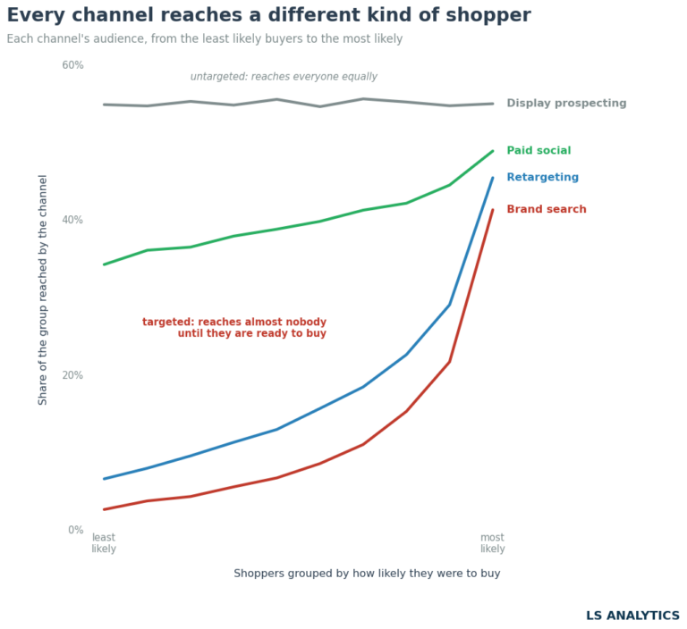
In our simulation, display reaches everyone at roughly the same rate, regardless of how likely they already were to buy. Paid social leans slightly toward people who were already a bit more likely to convert, and out of the four channels, it carries the biggest real effect. Retargeting only reaches people who already visited the site, which by itself marks them as close to buying, and what it adds on top of that is small. Brand search reaches almost nobody except shoppers who were already close to buying- people typing the brand name into a search engine because they had already decided- and what it adds on top is close to nothing. We defined those probabilities above, and now we will use them directly in the data structure we are building.
def intercept(t, reach):
    return brentq(lambda a: expit(a + t * intent).mean() - reach, -25, 25)

seen = pd.DataFrame(index=range(N))
for c, p in CHANNELS.items():
    a = intercept(p["targeting"], p["reach"])
    seen[c] = RNG.random(N) < expit(a + p["targeting"] * intent)

S = seenvalues
EFF = np.array([CHANNELS[c]["effect"] for c in CH])

dec = pd.qcut(intent, 10, labels=False)
grad = pd.DataFrame({c: pd.Series(S[:, j]).groupby(dec).mean() for j, c in enumerate(CH)})
The targeting part decides how much the channel cares about who it targets. Zero means essentially no targeting, while higher values mean a higher probability of targeting customers with high buying intent.
The last two lines sort shoppers into ten groups, from least likely to buy through most likely, and count what share of each group every channel reaches.
The above chart highlights how each channel works in the simulation. The steeper the slope, the more the channel’s audience was going to buy anyway.
The next step of the simulation solves every marketer’s deepest dream. Here, we decide each channel’s contribution.
def p_buy(mat):
    return np.clip(p_base + (mat * EFF).sum(1), 1e-6, 0.999)

p_actual = p_buy(S)
bought = RNG.random(N) < p_actual
p_buy determines each shopper’s chance of buying. It starts from p_base, the initial likelihood of making a purchase, and adds the effect of every ad they saw. Someone who saw paid social and retargeting gets both of those effects added on top of where they started. Someone who saw no ads keeps their original probability unchanged.
This gives us each customer’s probability of buying. And the last line is essentially a dice throw. For each person, we draw a random number, and if it lands below their probability, they buy. Someone with a 30% probability of buying will buy a product roughly 3 times out of 10.
At this point, we have defined the behaviour of both customers and marketing channels. Now we combine them to finish the simulated data. We will simulate each channel being switched off and on. This will let us see how much sales each channel actually caused to measure incrementality.
caused = {}
for j, c in enumerate(CH):
    off = S.copy(); off[:, j] = False
    caused[c] = (p_actual - p_buy(off))[S[:, j]].sum()
This part runs for all the channels and measures their effect on sales. With this information, we can explore the results and intricacies of the simulated world we created.
Last-click attribution vs true incremental sales
With the simulated data at hand, we can compare the conversions we would see using simple last-click attribution with the numbers we know the marketing activities actually caused.
This chart shows the difference between attribution and incrementality.
Every channel is clearly drastically overstated in the attribution reporting. As we discussed above, brand search and retargeting are clearly driving fewer incremental sales because they sit near the end of the decision funnel, reaching only customers with a high propensity to purchase. By the time either ad shows up, a potential customer has usually already decided, but the ad still gets credit for this decision. Brand search is attributed 1,920 sales against 24 it actually caused. Retargeting is attributed 1,825 sales against 143.
Paid social and display reach people with a lower baseline propensity to buy, which is why their incremental effect is larger. Paid social is attributed 2,861 sales against a real effect of 880. Display prospecting is attributed 2,031 sales against a real effect of 660. The gap between attribution and incrementality is still high, but lower than for brand search and retargeting.
This chart clearly shows the difference between the two ideas, and the differences here are high on purpose to highlight it.
Attribution counts presence. It looks at the sale, looks backwards across the customer path and assigns credit to the channels that we observed and tracked on the customer journey. Of course, different attribution models weigh channels differently, but they still have drawbacks. And not every touchpoint is always measured on the customer journey.
That’s where incrementality comes into play. It asks a narrower, harder question. It asks what would have happened if a given channel stopped running. Whatever sales disappear when the channel disappears, that’s what the channel was actually worth. We want to answer what conversion a given channel or marketing activity caused. Or, in other words, what would have happened if a given promotion or channel hadn’t appeared. This is a different question than attribution, and answering it requires a different set of tools from the causal inference universe.
The difference in our example is large. The attribution report recorded 8.6k sales, but only 1.7k were incremental. The remaining almost seven thousand sales would have occurred even without any active marketing promotion activities. This doesn’t mean we have to switch off all marketing activities, since we usually don’t know which conversions were incremental and which weren’t. But it’s a good case to think a lot about actual incrementality.
This doesn’t make attribution useless. It answers a question quickly, which is exactly what a marketing team needs to keep campaigns running week to week. The problem is not the tool. It is asking the tool to answer a question it was never built for. Attribution needs to be paired with incrementality to drive the best marketing results.
How to measure incrementality with a geo experiment
Everything so far depends on knowing the answer in advance. We wrote the rules so we could switch a channel off and measure what changed. This never happens in the real world. The only way to measure incrementality is via different tests and causal inference applications. We won’t cover those approaches comprehensively here, as they could easily fill hundreds of articles like this. Nevertheless, we will focus on a simple example showing, in a simplified way, how to measure incrementality using geotesting.
The most obvious way to measure incrementality is through randomised experiments, or A/B testing. We split the target population into two or more groups, give the treatment to one, and compare the results. Because of randomisation, the only difference between the groups can be attributed to the treatment itself, making it easy to measure the incremental effect.
Such tests are not always possible in marketing, especially when we are not testing activities that directly target individuals. Without being able to split customers into random groups, traditional A/B testing isn’t possible. This often happens with different types of above-the-line advertising and promotions that target a broader audience.
For that reason, we often use geo-testing, which randomly splits different regions, not customers. We can select a channel, choose which geographical regions to include and which to exclude, and measure the effect. With proper randomisation, the difference between regions with the channel switched on and those with it switched off gives the incremental effect of a given marketing action.
The following example will be very simple. We will take twenty markets; ten will randomly continue to receive brand search, and in the remaining ten this channel will be switched off. After some time, we will compare sales between the two sets of regions. The difference in sales between the two groups will give us the incremental effect of brand search. This simple simulation is being done by the code below.
MKTS, PRE, POST = 20, 60, 30
scale = RNG.uniform(600, 1400, MKTS)
treat = np.zeros(MKTS, bool); treat[RNG.permutation(MKTS)[:10]] = True
season = 1 + 0.12 * np.sin(np.arange(PRE + POST) / 9.0)
bs_share = CHANNELS["Brand search"]["effect"] * CHANNELS["Brand search"]["reach"] / bought.mean()

rows = []
for m in range(MKTS):
    lam = scale[m] * season * bought.mean() * 40
    off = np.r_[np.zeros(PRE), np.full(POST, bs_share if treat[m] else 0.0)]
    rows.append(RNG.poisson(lam * (1 - off)))
We simulated ninety days of daily sales. For sixty days, there is business as usual. Then, the experiments started, and we recorded 30 days of sales after brand search was switched off in ten randomly selected markets. Putting all the results in one dataframe allows us to measure average sales in both groups and compute the test results.
geo = pd.DataFrame(np.array(rows).T, columns=[f"m{m}" for m in range(MKTS)])
geo["day"] = np.arange(PRE + POST)
tcols = [f"m{m}" for m in range(MKTS) if treat[m]]
ccols = [f"m{m}" for m in range(MKTS) if not treat[m]]
geo["treatment"] = geo[tcols].sum(axis=1) / geo.loc[:PRE-1, tcols].sum(axis=1).mean() * 100
geo["control"]   = geo[ccols].sum(axis=1) / geo.loc[:PRE-1, ccols].sum(axis=1).mean() * 100

gap = (geo.loc[PRE:, "treatment"] - geo.loc[PRE:, "control"]).mean()
pre_gap = (geo.loc[:PRE-1, "treatment"] - geo.loc[:PRE-1, "control"]).abs().mean()
This results in an average gap after the brand search was switched off of -0.64% of baseline sales, which is basically no effect. The following chart shows this clearly.
Sales in both regions trended the same way before the experiment, which is a good sign that the randomisation was done properly. Any difference in trends between those groups would indicate that a selection wasn’t random. We can also see no gap after the experiment started. If brand search had an effect, switched-off markets would decrease more than markets with the campaign still running. This clearly shows that brand search is not driving incremental sales and calls into question investment in this channel. Unless there are other strategic reasons to keep branded search, running this channel is not the most efficient use of limited marketing resources.
Of course, in reality, such a test is much more complicated, but it gives us a good indication of how to use testing to measure incrementality. Experiments are messier and more complex in practice, but every business needs to know how it spends money and what effect it has.
Why marketing measurement needs causal inference
Let’s go back where we started. A simple dashboard starts by ranking channels by conversions. And such data is accurate and shows what actually happened. However, we have to remember what this data was designed to show. Correlational data, regardless of how well it is presented, focuses on what happened alongside the sale. It doesn’t tell us what actually caused a given conversion. From correlational data alone, we will never know the incremental effect of marketing activities.
More tracking doesn’t close that gap. Longer attribution windows, better cross-device matching, a smarter model in place of last-click- none of it changes what kind of question the data can answer. To answer the causal question, we need different tools, and that’s where causal inference comes into play.
None of this argues for abandoning attribution. It answers an important question, quickly and across every channel at once, and that’s genuinely useful for running a business. What it can’t do is tell us whether any activity is worth the money, because that was never the question it was built to answer.
The two need to work together: attribution for the daily view, and periodic incrementality tests to check that the daily view still means something.