Many product decisions in online companies rest on A/B tests. We show one version of the website to one group of customers and another to another. Then we compare what each group does and decide which version to roll out. The same principle applies to all randomised experiments. Before trusting that comparison, we first run one check: sample ratio mismatch (SRM).
The comparison is fair only when the two groups are alike, which random assignment achieves. Each website visitor gets a virtual coin flip that decides whether they belong to the treatment or control group. As a result, both groups have the same mix of customer characteristics, from demographics and past transactional behaviour to unmeasurable factors such as character and social background. These factors should be essentially the same across both groups. In an A/B test, the only difference between groups is the treatment itself, which is what makes randomised experiments such a powerful tool for measuring causal effects.
Sample ratio mismatch (SRM) warns that this balance is broken. For example, in an experiment with a planned 50/50 split, one group can have noticeably fewer people than the other. This indicates a problem with experiment design.
If sample ratio mismatch happens, the two groups stop being similar, which invalidates A/B test results. That’s why checking it matters, but experimentation often neglects it.
In the following article, we will explore sample ratio mismatch in more depth. We will see how a simple statistical check catches the problem, how to trace it to the missing users, and how to recover the true result.
What is sample ratio mismatch?
Sample ratio mismatch happens when the number of units in each A/B test group deviates from the planned split by more than chance can explain.
The last part is important because chance always plays a role in random selection. When you flip a coin 1,000 times, you will rarely get exactly 500 heads and 500 tails. We might get 509 or 492, and no one would call the coin biased. But with 600 heads, the case would be different, since that result would seem very unlikely.
A/B testing works in the same way. When splitting 200,000 users 50/50, a result like 100,150 vs 99,850 is plausible. A result like 98,000 vs 102,000 is way less likely. Random assignment would rarely produce it on its own, so something in the setup is wrong.
The split we want to achieve doesn’t have to be 50/50. We can split the group of interest in any other way, like 90/10, 80/20 and so on. The sample ratio mismatch applies to any random split. In all cases, we want to know one thing: are the actual counts what we expect from the experiment plan?
Why sample ratio mismatch breaks A/B test
An A/B test is designed to answer what happens when the same groups of people (or other units of experiment) receive different treatments. Random assignment should ensure we compare the same population and that the only difference between groups is the treatment itself. Sample ratio mismatch would break this assumption.
The problem lies in who gets misallocated to treatments. With sample ratio mismatch, the distribution of variables between treatment and control groups may no longer be equal, invalidating the purpose of the randomised experiment.
In technical terms, sample ratio mismatch breaks the exchangeability assumption. It assumes the treatment and control groups are identical in all baseline characteristics, so switching assignments would yield the same expected outcomes. For example, technical errors in the checkout flow design can add to the treatment group only customers who already added an item to the basket.
In that case, the control group includes all user types, while the treatment group excludes casual browsers who left before adding an item to the cart. It is artificially weighted heavily toward high-intent buyers. And we can never be sure that imbalance wasn’t created on some dimension we can’t even measure. Sample ratio mismatch doesn’t tell us what caused the imbalance or whether it happened at all. Still, it’s an important alert signal that something is wrong with the random assignment and that it undermines trust in the experiment’s results.
The case: a checkout A/B test
In the following parts of this article, we will use a simulated business example to show sample ratio mismatch in practice. An online shop redesigns its checkout page and tests it against the current version. The setup is as follows:
- 200,000 users reached over 14 days.
- An assignment service splits them 50/50
- The A/B testing platform counts a user when an “exposure” event fires in the browser.
On day 5 of the test, the developers released an update to the treatment version. The update changed the exposure event so it fires only after a new page component has loaded. On some devices, the component loads slowly, and some users left checkout before finishing the shopping process.
The redesign itself does not affect conversion. We built the data that way on purpose, so we know the right answer is zero.
The results
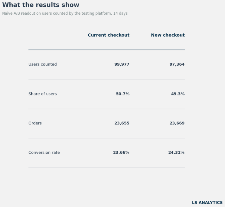
After 14 days, we obtained the following results from the experiment.
The new checkout converts 0.65 percentage points higher, with a relative lift of +2.7%. The 95% confidence interval ranges from +0.27 to +1.03 points, and the p-value is 0.0007. By all metrics, the experiment was successful.
After seeing those results, the company decided to roll out the redesigned checkout flow to all of the customers. Before doing so, no one noticed the split between the two versions wasn’t perfectly even, so no one investigated further. Ultimately, it led to the wrong decision that could have been very costly.
How to detect Sample Ratio Mismatch: the chi-square test
What’s striking is how easy it is to avoid such mistakes, as it just requires running a simple statistical test. The standard way to check for sample ratio mismatch is the chi-square goodness-of-fit test.
The idea is simple. It compares the counts we would expect under the desired randomisation split with the counts observed in the experiment. The test then uses the chi-square distribution to assess how likely this difference is if the split were truly fair.
In our example, the experiment platform counted 197,341 users in total. We observed 99,977 users in the control group, and 97,364 in the treatment group. Based on a 50/50 split, we would expect 98,670 users in each group. Looking at the counts, each group has about 1,000 users more or less than expected.
Using the chi-squared test, we can assess whether such a difference is likely to occur by chance alone.
For each group, we take the distance from the expected count, square it, and divide by the expected count. Squaring makes large gaps count far more than small ones. Dividing by the expected count scales the gap to the test size. After all, a difference of 1,306 users means much more in a test of 2,000 people than in a test of 200,000.
Here is the full test output from running the test in the notebook. Control is the current checkout, and treatment is the new one.
Chi-square goodness-of-fit test: sample ratio mismatch
--------------------------------------------------------------
Group          Observed    Expected   Difference    Share
Control          99,977    98,670.5     +1,306.5   50.66%
Treatment        97,364    98,670.5     -1,306.5   49.34%
--------------------------------------------------------------
Total           197,341
Planned split                                        50% / 50%
Chi-square statistic                                     34.60
Degrees of freedom                                           1
p-value                                               4.05e-09
Threshold (alpha)                                        0.001
--------------------------------------------------------------
Result: SRM detected. Do not trust the results yet.
Reading this table is simple. It immediately tells us whether the sample ratio mismatch has been detected.
- Expected is what the planned split predicts for this total
- Difference is how far each group is from that figure.
- The chi-square statistic sums these gaps. Here it is 34.60.
- Degrees of freedom are the number of groups minus one.
- The p-value is the chance of a gap this large if users were really split at random. Here it is 0.000000004. A fair split would produce a gap this big about four times in a billion tests.
- The threshold is the cut-off p-value we use to decide whether we detect sample ratio mismatch.
Since the p-value is below the 0.001 threshold, we can conclude that such a split is very unlikely to occur by chance alone, implying the existence of sample ratio mismatch. Unfortunately, our A/B test data is unreliable and shouldn’t drive business decisions.
With sample ratio mismatch testing, it is common to use a stricter decision threshold to reject the null hypothesis than the standard 0.05. The reason is that the check runs on every test, often several times while it is live. With a 0.05 threshold, one healthy test in twenty would raise a false alarm. With multiple tests, 0.05 would trigger more false alarms, and many would be unjustified. Hence, a stricter threshold of 0.001 prevents this, keeps alarms rare, and forces us to treat each alarm seriously.
The test confirms that something is wrong, but it cannot say what went wrong, what users are missing, or how the results are biased. The next section goes beyond sample ratio mismatch testing and shows how to trace the problem to its source.
How to diagnose Sample Ratio Mismatch
The sample ratio mismatch test told us the random assignment wasn’t correct and that the experiment’s randomisation wasn’t set up properly. But instead of stopping here, we can dig deeper and see what we can salvage. Since we suspect a technical bug broke the randomisation, we can start by checking the data.
Split by device
Let’s start by running a chi-square test separately for user devices. We have data available for Android, iOS, and desktop.
Both desktop and iOS pass the test, meaning approximately 50% of users were assigned to the treatment group, and their p-values reflect that. On the other hand, Android fails the SRM test severely, with only around 47% of users in the treatment group.
The whole problem is limited to one device. This shows the assignment wasn’t broken universally, but rather caused by a technical error in the new version that behaves differently on Android.
Split by time
Next, we will rerun the test at the end of each day to isolate the problem to a specific time when the experiment was running. We can do it by checking the cumulative ratio of customers in the treatment group at the end of each day when A/B was live.
For the first four days, the split was close to 50%. On day 5, it started decreasing, and it kept decreasing until the end of the test. That date matches the update that was made during the test.
We now have a clear picture of what broke the experiment. After exploring the data further, we identified the device causing the problems and the likely cause of the broken data in this experiment. We can learn the first, and most crucial, lesson here. Introducing significant changes during the test is risky and can produce faulty data that invalidates much of the experiment.
Summary: How to fix sample ratio mismatch
Strictly speaking, we can’t repair data with a sample ratio mismatch. The missing users are gone, and the remaining users are no longer a fair comparison. We can either salvage part of the experiment or rerun it.
If the analysis isolates the problem to a specific data segment, we can drop it and analyse the rest. Here, that means removing Android users from day 5 onward in both the control and treatment groups. This change adds cost and risk, making the overall analysis difficult.
We lose a large chunk of data, and the answer no longer covers Android users. More importantly, it also relies on an assumption we cannot prove: that the bug affected nothing outside that segment.
Any experiment using only such a subsegment can be challenged. However, sometimes there is no other option, as rerunning fast might not be possible. Practical scenarios might not always align with the ideal case. Also, causal inference tools such as propensity score matching can help limit bias.
The only certain solution is to rerun the experiment. It costs time, but it is the only option that doesn’t depend on assumptions.
The real lesson from this case is about prevention, because every fix comes after the damage is done. That’s why it is very important to remember the following when running experiments:
- Run the SRM check on every test, every day.
- Never change one version while the test is live.
- Record users in the same way in both versions
- Check the split before you analyse the result.
In our example, the business was one decision away from rolling out a change that did nothing. The sample ratio mismatch check that would have stopped it is one of the simplest statistical tests. Running it can save us from wrong decisions and prevent losses that hurt our operations.