Estimating the effect of one variable on another is central to causal inference. However, observational data can make this challenging, especially when confounding variables are present.
The Backdoor Criterion, introduced by Judea Pearl, provides a systematic way to identify which variables you should control for to estimate a causal effect accurately.
In the following article, we will explain the Backdoor Criterion using real-life examples. We will simulate data for each of them and estimate the simple causal effect using regression analysis in Python.
What is a DAG? Drawing the map of causality
To fully understand the backdoor criterion, we must introduce causal diagrams. They are the backbone of Judea Pearl’s causal inference approach, and understanding the general concept is relatively straightforward and intuitive.
A Directed Acyclic Graph (DAG) is a tool for visualising and reasoning about causal relationships between variables. The main components of each graph are nodes and arrows. In a DAG, nodes represent variables and directed edges (arrows) represent causal effects.
The arrows explain the ‘directed’ part. What about acyclic? It’s also simple: the arrows can go only in one direction. DAGs have no feedback loops. Once arrows leave a node, there is no way to return to it. For now, this may sound abstract, but the examples below will clarify how graphs apply to discovering causal effects.
As usual, reality is much messier, and we will rarely have a straightforward way to estimate causal effects, especially with observational data. In such situations, DAGs become increasingly complex, and estimating causal effects requires conditioning on and accounting for other variables.
DAGs can have so-called backdoor paths, and one way to estimate causal impact is to apply the backdoor criterion. – O
The backdoor criterion: identifying control variables
The Backdoor Criterion is a rule that helps to identify which variables to control for when estimating a causal effect from observational data. Let’s start with the formal definition.
A set of variables Z satisfies the Backdoor Criterion relative to a treatment X and an outcome Y if:
1. No variable in Z is a descendant of X and
2. Z blocks every path between X and Y that contains an arrow into X
If these conditions hold, conditioning on Z allows us to estimate the causal effect of X on Y even from observational data. If these criteria are met, we can estimate the treatment effect as if we had data from a randomised experiment.
A backdoor path is any path from X to Y that starts with an arrow pointing into X, representing non-causal associations that could confound the actual causal effect.
This definition is even more abstract than that of DAGs, and I had considerable difficulty understanding the practical implications of these rules. However, practical examples make this easier to understand.
In practice, applying the backdoor criterion means adjusting for common causes (confounders) of both X and Y, while avoiding adjustment for variables affected by X (mediators) or influenced by both X and Y (colliders).
We will examine each situation using linear regression and simulated data in the examples below.
Case 1: Confounder bias in a job training program
Imagine you’re evaluating whether job training improves employee productivity. However, you did not conduct the job training on a randomly selected sample of employees. As a result, all employees could take part in the training.
This makes assessing the program much more difficult, as many factors can influence both productivity and participation in the training program.
A key problem is that more motivated employees are both more likely to attend training and to perform better, regardless of whether they receive training.
To simplify, we will measure the following three variables, represented in the simulated data below:
motivation = np.random.normal(0, 1, n)
training_hours = 0.9 * motivation + np.random.normal(0, 2, n)
productivity = 5 * training_hours + 3 * motivation + np.random.normal(0, 1, n)
data1 = pd.DataFrame({'motivation': motivation,
                                         'training_hours': training_hours,
                                          'productivity': productivity })
- Employee motivation – regardless of how it’s measured, for example, as a result of employee surveys
- TrainingHours – number of hours an employee spent in the training program
- Productivity
The data is constructed so that motivation affects both training hours and productivity, as shown in the DAG below.
In such a case, motivation acts as a confounder. We also hard-coded the actual effect of motivation on productivity as a 5-unit increase in productivity for each one-unit increase in training hours.
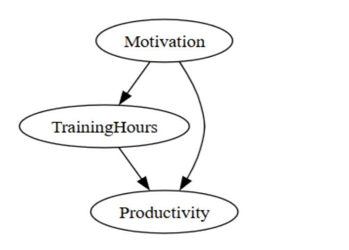
What is a confounder? It is a variable that influences both X and Y, potentially biasing the causal effect. It affects both the treatment and the outcome variable. I
In our case, motivation affects both training hours and productivity. How can we measure the causal effect of the training programs in such a case?
The most straightforward approach is to ignore motivation and estimate the effect of training on productivity. We can do it by running a regression with training hours as an independent variable:
## without adjustment
print("Naive regression without adjustment:")
naive_model1 = smf.ols('productivity ~ training_hours', data=data1).fit()
print(naive_model1.summary())

## with adjustment
print("Regression with adjustment for motivation:")
model1 = smf.ols('productivity ~ motivation + training_hours', data=data1).fit()
print(model1.summary())
Unsurprisingly, the results do not accurately reflect the treatment effect. According to this model, each additional hour of training increases productivity by 5.56 units. The treatment effect is 11% higher than the actual effect.
The difference might not be drastic, but it clearly shows that failing to adjust for the confounder (motivation) leads to a biased estimate of the treatment effect.
The effect is higher than the actual effect because more motivated employees are more productive and more likely to participate in the training program.
According to the Backdoor Criterion, to estimate the causal effect of Training Hours on Productivity, we need to block any backdoor paths from Training Hours to Productivity. The only backdoor path here is:
- TrainingHours <- Motivation -> Productivity
This requires controlling for motivation to isolate the actual effect of training. By conditioning on Motivation, we block this backdoor path.
Motivation is not a descendant of TrainingHours and blocks the non-causal path, so it satisfies the criterion above. To control for motivation, we will run another regression model that includes motivation as an additional variable.
This time, the treatment effect, represented by the coefficient on the training_hours variable, is much closer to the actual impact. The slight difference comes from including the random noise in the simulation.
By adjusting for the confounder, we estimated the treatment effect more accurately. We can solidify our knowledge by exploring a slightly more complex example with confounders.
Case 2: Confounding from seasonality and economic conditions
This time, let’s switch to the marketing world. We will examine whether increasing ad spend increases sales. However, isolating the effect of marketing spend on sales is complex.
Both general economic conditions and seasonal fluctuations can impact sales. After all, customers tend to spend more in periods of economic growth.
Additionally, seasonality can impact sales – for example, we tend to buy more ice cream in the summer, or heating bills are higher during the winter.
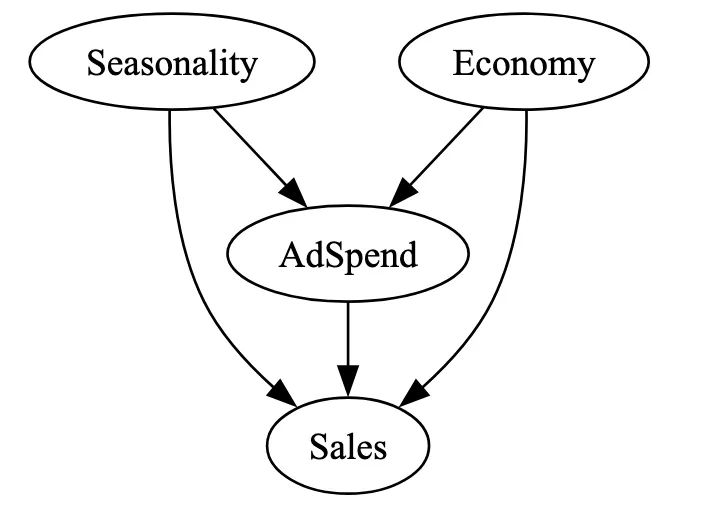
Let’s simulate our little scenario with the following code. Ad spend will affect sales. However, economic conditions and seasonality affect both advertising spend and sales, as shown in the graph below.
The actual effect of ad spend on sales is a 3-unit increase in sales for every one-unit increase in advertising spend.
seasonality = np.random.normal(0, 1, n)
economy = np.random.normal(0, 1, n)
ad_spend = 0.6 * seasonality + 0.4 * economy + np.random.normal(0, 1, n)
sales = 3.0 * ad_spend + 1.0 * seasonality + 0.5 * economy + np.random.normal(0, 1, n)

data2 = pd.DataFrame({'seasonality': seasonality,
                                          'economy': economy,
                                          'ad_spend': ad_spend,
                                           'sales': sales })
We already know that conditioning only on advertisement spend won’t accurately represent the treatment effect. Let’s confirm this with the following formula:
As expected, the naive approach inflates the actual treatment effect. This can be dangerous, as marketing managers may make incorrect budget-allocation decisions, resulting in excessive spending with no benefit.
As we already know, we must adjust for additional variables to uncover the true treatment effect. The first step is to identify all backdoor paths we need to control.
In our case, there are two backdoor paths from AdSpend to Sales:
- AdSpend <- Seasonality -> Sales
- AdSpend <- Economy -> Sales
By adjusting for both Seasonality and Economy, we will block both non-causal paths. Neither Seasonality nor Economy variables are descendants of AdSpend, so the adjustment satisfies the Backdoor Criterion.
To isolate the effect of advertising on sales, we will run a new regression model this time adjusting for both Seasonality and Economy:
## Naive (unadjusted) regression
naive_model2 = smf.ols('sales ~ ad_spend', data=data2).fit()
print("Unadjusted model:")
print(naive_model2.summary())

## Adjusted regression
model2 = smf.ols('sales ~ ad_spend + seasonality + economy', data=data2).fit()
print("\nAdjusted model:")
print(model2.summary())
As shown below, this model accurately identifies the effect of advertising spend. As in the example above, the slight difference is due to random noise.
This example illustrates a common business pitfall: analysts attribute higher sales to ads when external factors drive both ads and sales. Again, adjusting for confounders helps us to estimate the causal effect correctly.
Case 3: Mediator bias in an email campaign
Now, let’s imagine we are studying the impact of a personalised email campaign on user purchasing behaviour in the e-commerce setting.
After sending the emails, we track engagement metrics, including click-through rates, time spent on the website, the number of product pages visited, and interactions with recommended products.
These metrics measure the level of attention and interest the user shows for the platform after receiving the email. We also measure buying behaviour on our website, as the ultimate goal of our campaign was to increase product sales.
We have both engagement and sales data, and our goal is to determine whether the email campaign increased sales. The following graph represents the situation.
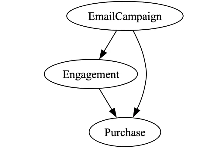
The following code will simulate our data. Note that the actual effect of the email is not directly visible in the code below. This is because purchase depends on both emails and engagement. Engagement is also affected by emails. Hence, we can distinguish two ways in which email affects spending:
- Direct effect – email campaign -> purchase
- Indirect effect: email campaign -> purchase -> engagement
n = 1000
email = np.random.binomial(1, 0.5, n)
engagement = 0.8 * email + np.random.normal(0, 1, n)
purchase = 1.2 * engagement + 0.5 * email + np.random.normal(0, 1, n)

data3= pd.DataFrame({'email': email,
                                         'engagement': engagement,
                                         'purchase': purchase })
Based on this, we can see that the simulated data is as follows:
- Direct effect: 0.5 units
- Indirect effect: email coeffcient on engament x enagament on purchase = 0.8 x 1.2 = 0.96
- Total effect of email campaign = 0.5 + 0.96 = 1.46
How should we approach measuring the total effect of the campaigns? In the examples above, we simply conditioned on all the available variables. Now let’s see what happens if we run a similar regression, adjusting for both engagement and the email campaign.
The coefficient of email in the model adjusted for engagement is 0.5. However, it does not capture the full effect of our campaign.
As we saw above, not. This regression captures only the direct impact of the treatment, which is lower than the total effect.
Adjusting in this manner may lead to severe business consequences, as we won’t be able to plan future marketing activities accurately.
What is happening here, then? Why didn’t adjusting for all available factors work, and did it used to work before?
It happens because we no longer have confounders. The engagement metric acts as a mediator, and variables in such a scenario require a different approach.
Let’s take a look at the causal path again. It looks like this:
- Email -> Engagement -> Purchase
- But also: Email -> Purchase
This means engagement is a mediator—it carries part of the campaign’s causal effect. A mediator is a variable that transmits part of the treatment’s impact on the outcome.
In our case, engagement acts as a mediator, as the email campaign directly causes it. The mediator also lies on the causal pathway between the treatment and the outcome.
From a practical perspective, we should never adjust for mediators, as it introduces so-called mediator bias, meaning we don’t capture the full treatment effect.
Including a mediator as a control variable means that our model estimates the direct effect of the treatment, not the total effect. This understates the email campaign’s actual impact and violates the backdoor criterion because it doesn’t capture the full causal effect.
Our goal is to assess the campaign’s overall impact on sales and purchases. To do this, we only need to run the regression with the email variable included.
As shown below, the email campaign’s effect is significantly larger and more closely resembles our simulated example (though it’s not identical due to random noise). We estimated the email campaign’s total effect accurately.
Adjusting for mediators is a hazardous practice that is often overlooked. For example, it’s pretty standard to use all available data to estimate the effect of a particular activity. As this case illustrates, that can lead to incorrect results and, in turn, wrong decisions.
It also shows that causal thinking helps us determine the effect accurately.
It also reminds us that thinking about the problem’s structure is just as important as running the analysis. Long story short – we can never adjust for mediators.
Case 4: Collider bias in a public health study
Our final example will introduce another type of bias and a situation where adjusting for a variable is worse than doing nothing. We will go into the public health realm.
Suppose we are analysing the relationship between compliance with a public health campaign (e.g., wearing masks or getting vaccinated) and an underlying health risk (e.g., chronic illness).
We will also include doctor visits as another variable in our model. Our goal is to estimate the effect of compliance on the risk of chronic illness.
The causal situation looks like this:
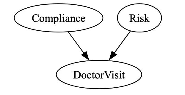
The data are simulated as follows. Both compliance and health risks lead to doctor visits. However, please note that there is no causal path between compliance and risk.
n = 1000
compliance = np.random.binomial(1, 0.5, n)
risk = np.random.normal(0, 1, n)
doctor_visit = 0.8 * compliance + 0.8 * risk + np.random.normal(0, 1, n)

data4= pd.DataFrame({ "compliance": compliance,
                                          "risk": risk,
                                           "doctor_visit": doctor_visit })
Now, let’s suppose we don’t account for the causal graph and include the doctor’s visit variable in our analysis. After all, why not use all the available data?
Using this approach, the doctor’s visit affects the health status. And this effect is quite significant.
Why does the inclusion of the supposedly unrelated variable lead to significant effects? It happens because the doctor’s visit acts as a collider. This is the last type of causal connection we’ll introduce in this article.
A collider is a variable that is causally influenced by two or more variables in a causal graph. As shown above, the arrows from two variables intersect at the doctor’s visit. A collider is the opposite of a confounder – it’s not causing other variables, but is caused by them.
When we condition on the collider as we did in the regression formula, we technically open a non-causal path between variables in our model. This creates a spurious effect that does not exist in reality. We call it a collider bias.
When two variables are truly independent in reality, conditioning on the collider creates a spurious connection between them that does not reflect the actual causal relationship.
Including the doctors’ visit variable in our analysis created a collider bias, as we ‘discovered’ an effect that is not causal. Compliance with health guidelines and disease risk are unrelated in the general population. But they become connected when we condition on doctor visits.
It happens because people who visit a doctor are generally at higher risk of disease. After all, relatively few healthy people want to see a doctor. On the other hand, people who are more compliant with public health measures are also more likely to visit a doctor, as they are concerned about preventing various diseases.
When we condition on visiting the doctor, we have two separate groups of people:
- Compliant with public health but without any diseases
- Sick people who are not compliant
Why would they visit a doctor?
If someone is compliant and visits the doctor frequently, they likely have a low risk (because their visits are for preventive care, not illness).
If someone is non-compliant but visits the doctor a lot, it’s probably because they’re sick and have a higher risk of chronic diseases.
Within the group visiting a doctor, compliance and illness risk become negatively correlated.
How to fix this error? The best approach is to do nothing, as including the doctor’s visit can lead to incorrect results. Let’s see what happens if we run a regression model without doctors – we try to predict the risk of disease by using only the compliance variable.
## Incorrect model (adjusts for collider):
naive_model4 = smf.ols('risk ~ compliance + doctor_visit',data=data4).fit()
print(naive_model4.summary())

## Correct model (does not adjust for collider and there's close to no association between compliance and risk):
model4 = smf.ols('risk ~ compliance', data=data4).fit()
print(model4.summary())
And this time our results are correct – the compliance coefficient is minimal with a large p-value. As our simulated data show, compliance does not affect disease incidence.
This example shows again that sometimes using too much data is worse than not using it at all. Conditioning on a collider can be very dangerous, as it may lead to incorrect conclusions that can, in turn, result in misguided decisions.
That’s why it’s essential to think about the structure of the data and potential relations between variables before adding them to our model. Only this approach will help us to discover the actual causal effect.
Backdoor criterion in practice: confounder, mediator, collider
Estimating causal effects with observational data is one of the most challenging tasks in analytics. Still, tools like DAGs and the Backdoor Criterion allow us to do it correctly.
In this article, we unpack how causal diagrams reveal pathways that can bias our
estimates, and how to block them by choosing which variables to adjust for in a regression model.
Let’s summarise what we have to do when we encounter the three main types of causal connections:
- Confounder – always block/add to the model
- Mediator – never block/do not add to the model
- Collider – never block/do not add to the model
We had one huge advantage – we already knew what the actual causal relationship between variables looked like. No analyst has this luxury. This is one of the biggest drawbacks of causal inference using DAGs.
We rarely know the actual causal diagram; we have to assume certain relationships based on our knowledge and experience.
We can approach this in many ways, which we will cover later, ranging from critical domain expertise and discussions with domain experts to the most advanced causal discovery techniques. Specialised tools and libraries can also help us estimate the strength of our assumptions and test them.
However, we must live with this drawback. And I have to highlight again – all analytics is about making certain assumptions. Before applying any causal model, even a simple regression, we must carefully consider what we want to discover and which variables make sense. Causal diagrams are the perfect tool for that.
References
Judea Pearl, Causal Inference in Statistics: A Primer, 2016
Pearl, J., & Mackenzie, D. (2018). The Book of Why: The New Science of Cause and Effect. Basic Books.