You might feel intrigued when a newspaper like the Washington Post runs an article about the statistical method. Statistical modelling isn’t usually the most exciting topic. However, in 2015 (yes, a long time ago), the Washington Post published an article describing the synthetic control group method. The fact that such a reputable source was discussing it hints at its importance. This article examines one of the most critical components of the causal inference arsenal: the synthetic control group.

This post is based on a seminal article by Alberto Abadie and Javier Gardeazabal, The Economic Costs of Conflict: A Case Study of the Basque Country. Their analysis not only examined the effect of terrorist activity on the Basque Country’s economic development but also set a new standard for causal inference research.
Terrorism activity in the Basque Country
Let’s start with a brief description of the analysed problem. In the middle of the 1970s, the Basque Country, one of the Spanish regions, was affected by terrorist activity conducted by the separatist ETA group. The group wanted to gain independence for the region from Spain. The authors of the article mentioned above evaluated the effect of violence on the Basque Country’s economic activity.
It is a perfect topic to explore from a causal inference perspective. As a first try, I tried to find an answer using the difference-in-differences method. This approach worked well when comparing the economic development in the Basque Country with that of similar regions, such as Catalonia. However, it does not work well when comparing several regions.
This is because the parallel trend assumption does not hold in our data. The chart below shows that distinct Spanish regions experienced varying economic growth rates before 1975. So we need another reliable method to detect a causal effect. The synthetic control group comes to the rescue.

What is a counterfactual in causal inference?
Before we explain this method, let’s consider what we want to accomplish. Given a set of different covariates X, how can we find a causal effect of activity T on outcome Y? In our case, we would like to determine the impact of terrorism activity on the Basque Country’s economic development.
Let’s call T the activity we want to study. Y is the outcome variable. The treatment effect (indicated by the letter delta) is defined by:

We aim to estimate the difference between the outcome variable in the presence of the activity and the same outcome variable without the activity. This is a bold formula, as we cannot observe the second part of the equation. The equation above contains the counterfactual term P(Y | T = 0). In causal inference, a counterfactual is a hypothetical scenario representing what would have happened if a particular event or condition had not occurred.
In the analysed problem, the first term of the equation contains actual data — the GDP of the Basque Country affected by terrorist activity. The counterfactual is a hypothetical Basque Country not affected by terrorist activity. To illustrate this, let’s consider a hypothetical scenario where the Basque Country did not experience terrorist activity. In this scenario, we can estimate the potential increase in GDP.
But at a given time, there is only one Basque Country. The counterfactual is just a hypothetical world. The equation above introduces two states of the world, two different realities. And we can observe only one of them — this is the fundamental problem of causal inference.
It is impossible to observe the same unit in two distinct versions of reality. However, we can still try to estimate it using available information and clever techniques. To answer our question, we need to establish what would have happened to the Basque Country if ETA had not started its violence in the middle of the 1970s. We have to find the counterfactual.
Our quest for the counterfactual leads us to the concept of a ‘clone’ of the Basque Country. This is not a search for an alternative reality but a pursuit of another unit in the real world that mirrors the Basque Country yet remains unaffected by the given activity. This approach brings us a step closer to our goal.
Of course, we will never find a perfect clone of any social entity. We have to estimate it. The key to many evaluation methods is to find a valid comparison. This group must be as similar as possible to the affected unit. If we achieve it, we will have the following groups:
- treatment group — a unit that was affected by the treatment
- comparison group- a unit that was not affected by the treatment but resembles the treatment group in all other criteria
We assume the treatment group would have the same outcome variable values as the comparison group without treatment (because they are identical). Thus, any difference between the two groups after treatment must have occurred solely because of it. This approach allows us to determine the causal effect of a given phenomenon.
This idea is simple, but we still have a lot of work to do. How can we find the ideal comparison group? The optimal approach is to conduct random experiments, which is not feasible in numerous real-world settings. We must search for the next best solution.
All non-experimental approaches require us to investigate a particular issue and review existing information to find comparison units that resemble the affected group. We already examined the difference-in-differences method; now, it’s time to explore the synthetic control group.
Choosing the donor pool
What would be the best comparison group to estimate the causal effect of terrorism activity on the Basque Country’s economy? We have already answered this question: other Spanish regions. We have data about their GDP per capita over the years. The remaining task is determining a method for combining them into a single entity. As we saw earlier, we cannot use difference-in-differences because we lack parallel trends.
But we can use a synthetic control group! This method lets us create a weighted combination of the comparison groups to form the synthetic control group. We will combine the data from many potential comparison units into one. Those will be part of the so-called donor pool.
All we have to do is weight each unit, and the combined weight should create a comparison group that resembles the treatment group as much as possible. We have to make them comparable in the pre-treatment period.
Synthetic control models optimally choose a set of weights which, when applied to a group of corresponding units, produce an estimated counterfactual to the unit that received the treatment.
To create a synthetic control group, we can only look at the pre-treatment period because that is when the units are expected to be as similar as possible.
To evaluate the treatment effect, we can compare the outcome variable in the treatment group to the values observed in the synthetic control group. The former is our counterfactual — it is a proxy to estimate what would have happened to the treatment group had the event of interest not occurred.
For the Basque Country problem, we have all the ingredients needed to apply the method. We have data on the Basque Country and all the other regions in the donor pool. Now we have to find a way to combine the remaining areas to create a group that resembles the pre-1970s Basque Country as closely as possible.
How do we create a synthetic control group?
We are almost there. Let’s summarise the approach we have taken so far. To create a synthetic control group, we should:
- Define our donor pool
- Combine the donor pool units into one to resemble the treatment group before the treatment
- Calculate the treatment effect
We have already defined the donor pool. Now, the crucial step is ahead of us. How can we combine the remaining Spanish regions to create a synthetic Basque Country? To do this, we must determine each region’s weight. Those weights have to resemble the pre-treatment GDP trend in the Basque Country. Fortunately, we already have statistical methods we can apply — the good old linear regression.
We can regress the GDP per capita in all Spanish regions on the Basque Country. In such a regression, the GDP of all other provinces is an independent variable, and the Basque Country’s GDP is the dependent variable. I’m reducing the details here, and you can find numerous resources that explain this approach in more detail, with statistical and technical information. Since we want to apply this approach, let us focus only on the necessary aspects. We will use the most straightforward (but still powerful) approach to see the power of this method.
We will use the Basque dataset as in the previous difference-in-differences study. Below is the data describing GDP per capita in a given Spanish region in a given year. To calculate the synthetic control group we will use only data points from 1975:

First, we must transform the data to build a synthetic group. Then we pivot it from the panel structure. Each region has to be stored in a separate column. Rows will indicate each year, with GDP as a value. You can do this quickly with pandas pivot.
regions_pre = data_pre.pivot(columns='regionname', values='gdpcap', index='year')
regions_pre.head()
The transformed dataset looks like this:

Another transformation we need to make is to separate the dependent and independent variables. We must store the Basque Country in a separate series and remove it from the table above.
basque_pre = regions_pre['Basque Country (Pais Vasco)']

regions_pre.drop('Basque Country (Pais Vasco)', axis='columns', inplace=True)
And the data is ready. If the values were on a different scale, we would have to standardise them, but it is not needed here as the GDP is on a similar scale across all regions.
Let’s build the first synthetic control group. We will start with a simple linear regression. It will give weights to each region to minimise the sum of squared errors between them and the Basque Country. Since we want to make predictions, I will use the scikit-learn library.
from sklearn import linear_model

linear_reg = linear_model.LinearRegression().fit(regions_pre,basque_pre)
Voilà, the model is already created. Now, we can apply it to our original dataset. We have to make another pivoted table. This time with all the years, but still without the Basque Country (as we can’t use it for prediction):
data_all_without_basque = data.pivot(columns='regionname',values='gdpcap', index='year')
data_all_without_basque.drop('Basque Country (Pais Vasco)', axis='columns', inplace=True)

synthetic_control_linear = pd.DataFrame(linear_reg.predict(data_all_without_basque))
synthetic_control_linear.index = data_all_without_basque.index
Finally, we apply the synthetic control group results to our main table, which includes the Basque Country. We will use this structure to calculate the treatment effect.
data_all_regions_pivot = data.pivot(columns='regionname',values='gdpcap', index='year')

data_all_regions_pivot['Synthetic_Control_Group_linear'] = synthetic_control_linear

The last column in the table above contains the synthetic control group prediction. We created a linear combination of all regions that should resemble the Basque Country as closely as possible.
Or maybe it’s too close? When we compare values between 1955 and 1975, we find that the synthetic control’s GDP per capita is almost identical to the Basque Country’s. It indicates overfitting. Before jumping to conclusions, we can finally see trends in the synthetic control and the Basque Country.

It looks like I did something wrong. Since 1975, the Basque Country has had a much higher trend than the synthetic control group. The overfitting indeed occurred. Our synthetic control group was too good before the treatment — it just mimics the behaviour of the Basque Country but can’t generalise well. We have to restrain linear regression.
This picture shows two important things. First, better tools exist to create a synthetic control group than standard linear regression. Second, to evaluate the results, we must apply domain knowledge, compare it with other methods (like difference-in-differences), and use common sense. We must verify any strange results, such as those above.
Constraining the weights with ridge regression
We are back at the drawing board. There are many ways to prevent linear regression from overfitting. The most common and powerful are ridge and lasso regression. Both use a regularisation parameter that keeps the weights from getting too high.
Ridge regression shrinks the parameters, while lasso goes further and sets some to zero. I will use ridge regression, as even the least similar region can contribute slightly to the synthetic control group weights. We can build a ridge regression with scikit-learn:
ridge_reg = linear_model.RidgeCV(cv = 5).fit(regions_pre,basque_pre)
I used 5-fold cross-validation here, which chooses the optimal regularisation parameter. After repeating the transformation we did for the linear regression above, we ended up with a new solution:

It looks much better now. The fit pre-1975 is not perfect, but the synthetic control group resembles the Basque Country. After 1975, the Basque Country decreased significantly compared to the control group.
The synthetic control group shows what would have happened to the Basque Country had the ETA terrorist activity not occurred. The difference between the blue and orange lines is the treatment effect — the loss of GDP per capita in the Basque Country caused by terrorist activity.
Let’s explore the synthetic control group more before calculating the treatment effect. We can examine the weights for each region.

Some regions contribute positively, while others contribute negatively. It raises an important question: Can we assume that some areas contribute negatively to creating synthetic control groups? Wouldn’t it be more appropriate to constrain each weight to be between 0 and 1?
Abadie, Diamond, and Harmuller solved this issue in the 2010 article. They applied the optimisation constraints to restrict the weights in this way. I recommend reading this article to better understand their approach.
Since then, a few libraries have implemented the synthetic control group method. I won’t implement this optimisation here, as it would not significantly expand our knowledge of this technique or enhance the model in the Basque Country scenario.
Calculating the treatment effect
As we established earlier, the synthetic control group is the counterfactual. We assume the treatment group would have had the same outcome variable values as the control group if the event had not happened.
To estimate the effect of terrorist activity, we can compare the post-1975 GDP in the Basque Country to the synthetic control group. Let’s plot the differences.

After 1975, the Basque Country’s GDP was nearly one unit lower than it would have been without the terrorist activity. Throughout the 1980s, this gap remained wide and only began to narrow in the 1990s. It demonstrates the potent impact of terrorism and the extent to which the violence has impacted this region. The rebound in the 1990s is related to the peace process that ended the streak of violence.
We also estimate the average effect of terrorist activity by comparing average GDP per capita between the two groups for the post-1975 period.
data_post_75 = data_all_regions_pivot[data_all_regions_pivot.index >= 1975]

avg_gdp_diff = np.mean(data_post_75['Synthetic_Control_Group_ridge'])  - np.mean(data_post_75['Basque Country (Pais Vasco)'])
The code above shows that, on average, terrorism reduced the Basque Country’s GDP per person by 0.84 units.
The impact of lost opportunities is significant and shows that combating terrorism is crucial to maintaining good prospects for economic prosperity. This result is similar to what we obtained in the difference-in-differences estimation with Catalonia, which supports our initial hypothesis that the two regions were closely comparable before treatment.
Validating results with a placebo test
Before we conclude, let’s address a crucial question: How reliable are these results? Could they be mere chance? The synthetic control group method offers a straightforward way to calculate our confidence in the obtained results. We do this through a placebo test.
The objective is similar to the placebo test in clinical trials. It involves applying a synthetic control group to a set of fake treatment units that did not get the treatment but are treated as if they did. By comparing the treatment effect in placebo units with the outcome in the affected unit, we can ascertain the statistical significance of the event of interest. The step-by-step algorithm for conducting a placebo test is as follows:
- Specifying a placebo unit — in our case, we will iteratively treat each region as the affected group.
- Constructing the synthetic control group — at this step, we will create a synthetic control group as we did for the Basque Country, but we will use the placebo unit as the target region.
- Calculating the treatment effect — the difference in GDP for each person between the synthetic control group and the placebo region.
- Repeat steps 1–3 for all regions.
- Calculate the statistical significance of the original synthetic control group by measuring how often the GDP difference in the placebo regions was greater than in the actual control group.
It is helpful to create a function to calculate a synthetic control group since we will have to repeat this process a few times. I will package the steps above into a function so we can select different regions as the affected units. I am just an analyst, not a programmer, so please forgive me if it’s not the most optimal way (but it works, so we’re good 🙂 ).
def synthetic_group_ridge_regression(data_all = data , data_pre = data_pre, target = 'Basque Country (Pais Vasco)'):

    regions_pre = data_pre.pivot(columns='regionname', values='gdpcap', index='year')

    target_pre = regions_pre[target]

    regions_pre.drop(target, axis='columns', inplace=True)

    ridge_reg = linear_model.RidgeCV(cv = 5).fit(regions_pre,target_pre)

    data_all_without_targed = data.pivot(columns='regionname',values='gdpcap', index='year')

    data_all_without_targed.drop(target, axis='columns', inplace=True)

    synthetic_control = pd.DataFrame(ridge_reg.predict(data_all_without_targed))

    synthetic_control.index = data_all_without_targed.index

    data_all_reg_pivot = data.pivot(columns='regionname',values='gdpcap', index='year')

    data_all_reg_pivot['Synthetic_Control_Group'] = synthetic_control

    data_all_reg_pivot['gdp_diff'] =  data_all_reg_pivot[target] - data_all_reg_pivot['Synthetic_Control_Group']

    return data_all_reg_pivot[['Synthetic_Control_Group', 'gdp_diff']]
The function returns a data frame with synthetic control group estimates and the difference between them and the actual values in the target region.
The code below adds one additional caveat we haven’t discussed yet. It excludes regions with a poor pre-treatment synthetic control group fit, giving us more stable results. We can follow the procedure presented in Abadie (2010), and excluding all regions for each MSE was more than five times higher than in the Basque Country.
data_all_regions_pivot_pre_75 = data_all_regions_pivot[data_all_regions_pivot.index < 1975]

basque_mse = np.mean((data_all_regions_pivot_pre_75['Basque Country (Pais Vasco)'] -  data_all_regions_pivot_pre_75['Synthetic_Control_Group_ridge']) ** 2)
This additional condition lets us include only placebo units with a solid pre-treatment fit. We can now actually execute the test. In this step, we must follow the placebo test procedure by running the function many times, each time selecting a different region as if it were affected by ETA terrorist activity.
The placebo test excluded only one region, indicating that the pre-treatment fit was good for all units.
After executing the code outlined above, we obtained a list of data frames containing placebo synthetic control groups. The placebo test, in its simplest form, follows a straightforward procedure.
Let’s plot the GDP difference between the placebo regions and the one we obtained from the Basque Country’s synthetic control group.

It is immediately apparent that the effect visible in the Basque Country is very unusual. The placebo regions did not have an immediate negative impact of this magnitude, but the actual synthetic control group quickly became intensely different from the placebo units.
We can confirm this visually by calculating the p-value for the synthetic control group. There is no one correct option for calculating the p-value of the synthetic control group method. For this exercise, I used the following procedure.
We will iterate over each post-treatment year, from 1975 to 1997. Each year, we will calculate the difference in GDP between the Basque Country and the synthetic control group. We will then iterate over each placebo region with its synthetic control group and calculate the GDP difference for this year.
As a result, we will store a boolean variable as True when the placebo effect is larger than the effect obtained in the Basque Country and False otherwise. We will repeat this procedure for each year and each placebo group.
diff_list = []

for year in range(1975, 1998):

    for i in range(len(df_list)):

        basque_gdp_diff = data_all_regions_pivot[data_all_regions_pivot.index == year]['gdp_diff'].iloc[0]

        gdp_diff_placebo = df_list[i][df_list[i].index == year]['gdp_diff'].iloc[0]

        test_cond = gdp_diff_placebo < basque_gdp_diff

        diff_list.append(test_cond)
To calculate the p-value, we only need the average of diff_list. It calculates the proportion of times when the placebo effect was more substantial than the effect obtained in the Basque Country synthetic control group.
After calculating the average, we obtained the following results:

The p-value is below the standard threshold of 0.05, indicating that the effect observed in the Basque Country study is unusual. We can reject the null hypothesis that terrorism activity did not negatively impact Basque Country GDP per capita.
Summary
The article shows the power and usefulness of the synthetic control group. It is one of the best tools in the causal inference arsenal because it allows us to create a counterfactual without assuming parallel trends. It’s particularly useful when traditional experimental methods like randomised controlled trials are not feasible or ethical.
The method is not perfect. Because it constructs a control group from historical data on untreated units, it assumes that relationships between covariates and outcomes remain stable over time (in the absence of treatment). Additionally, we can only be somewhat sure that the event of interest is the only thing affecting the outcome in the affected group. This assumption requires substantial domain knowledge and understanding of the analysed problem. Hence, we can’t apply it as a black-box algorithm to solve these issues.
This approach is beneficial for evaluating different interventions at the aggregated level. Applying synthetic control at the level of specific regions and countries is the best application of a synthetic control group. The relative ease of this method makes it much more popular. I regret learning about it only recently, and I hope this article adds a small contribution to the popularisation of the synthetic control group.
References:
Abadie, Alberto & Gardeazabal, Javier. (2003). The Economic Costs of Conflict: A Case Study of the Basque Country. American Economic Review. 93. 113–132. 10.1257/000282803321455188.
https://mixtape.scunning.com/10-synthetic_control
https://matheusfacure.github.io/python-causality-handbook/15-Synthetic-Control.html